How can I solve an equation with symbolic coefficients?

Question

I want to try to solve the following

 a x^(17/6) - b x^2 - 1 == 0

where a and b are variable coefficients (which are very small and positive).

I cannot get an analytic solution (not surprised), but NSolve is not doing the job for me. I am a novice to Mathematica; is anyone able to do NSolve for x on Mathematica and get a numerical result?

Answer 1

One thing that you could do is to rescale your equation:

Clear[x, ξ, eq1, eq2, A];
eq1 = a x^(17/6) - b x^2 - 1 == 0
eq1 /. x -> A*ξ // PowerExpand

The result is:

-1 - A^2 b ξ^2 + a A^(17/6) ξ^(17/6) == 0

Choose A such that the factor in front of the largest power is unity:

s1 = Solve[a A^(17/6) == 1, A][[1, 1]];
Simplify[(eq1 /. x -> A*ξ /. s1) /. b -> c*a^(12/17), {A > 0, a > 0, b > 0}]

where c = b/a^(12/17). Now you have an equation with a single parameter, easy to solve. Here it is:

1 + c ξ^2 == ξ^(17/6)

You can define the interval of its variation, I cannot do that. For this reason to give an example I suppose that c varies from 0 to 2. Let us look at the solution. Evaluate this:

Plot[{1 + \[Xi]^2, ξ^(17/6)}, {ξ, 0, 3}, 
  PlotStyle -> {Red, Blue}, 
  AxesLabel -> {Style["\[Xi]"], 
     Row[{Style["1+\!\(\*SuperscriptBox[\(\[Xi]\), \(2\)]\), ", Red], 
     Style["\!\(\*SuperscriptBox[\(\[Xi]\), \(17/16\)]\)", Blue]}]}]

You will see this image:

There is a solution in the vicinity of ksi=1.5. Now we can make a list of numeric solutions of this equation. Evaluate this:

lst = Table[{c, FindRoot[1 + c*ξ^2 == ξ^(17/6), {ξ, 1.4}][[1, 2]]}, {c, 0.1, 2, 0.01}];   

By plotting this list, one finds the dependence of solutions upon the value of the parameter c. Evaluating this:

ListPlot[Select[lst, #[[2]] ∈ Reals &], 
   AxesLabel -> {Style["c", 14], Style["ξ", 14]}, 
   AxesOrigin -> {0, 0}]

One gets the following plot:

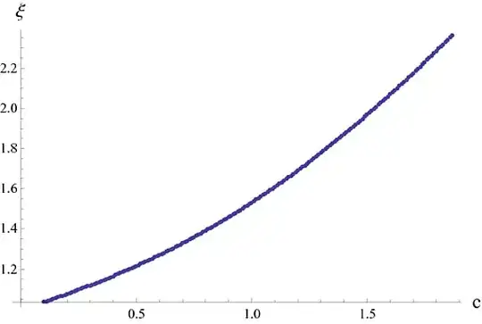
This is already the solution you are looking for. You can do somewhat more, however. If one fits the solution by some simple function on this interval of c, one finds (though approximate) an analytical and accurate solution that can be used in further analytical calculations, if any:

ft = Fit[Select[lst, #[[2]] ∈ Reals &], {1, c, c^2}, c]

which yields this:

1.00914 + 0.292415 c + 0.231262 c^2

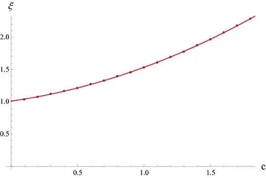
This is your solution. To see, how accurate it is, evaluate this:

Show[{
   ListPlot[Select[lst, #[[2]] ∈ Reals &], 
      AxesLabel -> {Style["c", 14], Style["\[Xi]", 14]}],
   Plot[ft, {c, 0, 2}, PlotStyle -> Red]
}]

You will obtain the following plot:

Have fun.

Answer 2

Geometrically, the locus of $(x,y)$ for which $a x - b y - 1 = 0$ is a line orthogonal to the vector $(a, -b)$, because the equation can be written $(a,-b)\cdot (x,y)=1$. This invites us to pose the problem as a geometric intersection:

Find all points of intersection of the line $a x - b y - 1 = 0$ and the curve $t\to (t^{17/6}, t^2)$.

Because this curve (clearly) is an arc starting at $(0,0)$ and rising at a rate of $O(x^{12/17}) \lt O(x)$ and the line (also clearly) has positive slope and negative intercept when $a\gt 0$ and $b\gt 0$, it is geometrically evident that a unique point of intersection exists. If you're unconvinced, or just want to appreciate the solutions a little better, you may use Manipulate to explore the situation in terms of $a$ and $b$. ContourPlot is good for showing functions given in implicit form (like $a x - b y - 1 == 0$) and ParametericPlot is good for plotting parameterized curves. Thus:

h[a_, b_] := Block[{x}, x /. FindRoot[a x^(17/6) - b x^2 - 1 == 0, {x, 10^12}]];
Manipulate[
 u =  h[a, b];
 Show[
  ContourPlot[a x - b y, {x, 0, 200000}, {y, -10, 5000}, Contours -> {1}],
  ParametricPlot[{t^(17/6), t^2}, {t, 0, 300}, PlotStyle -> {Thick, Red}], 
  Epilog -> {White, PointSize[0.015], Point[{u^(17/6), u^2}]}],
 {a, 10^-6, 1}, {b, 10^-6, 1}
 ]

(FindRoot works just fine to obtain a numerical solution--shown as a white dot--provided we ask it to start near infinity in its search.)

Now that we know there is a unique solution, use Solve to obtain an analytic expression. Let's encapsulate this in a function of the variable coefficients:

f[a_, b_] := Evaluate[Flatten[x /. Solve[a x^(17/6) - b x^2 - 1 == 0, {x}]]]

This function returns a list of $17$ Root objects; for instance, the first in the list is

$$\text{Root}\left[-1-6 b \text{$\#$1}^2-15 b^2 \text{$\#$1}^4-20 b^3 \text{$\#$1}^6-15 b^4 \text{$\#$1}^8-6 b^5 \text{$\#$1}^{10}-b^6 \text{$\#$1}^{12}+a^6 \text{$\#$1}^{17}\&,1\right].$$

This is a perfectly good "analytic" expression. Moreover, because Solve guarantees that it will list its real roots first, this is the unique real root (when $a\gt 0$ and $b \gt 0$). We can plot it as a function of the coefficients $a$ and $b$ (although it takes some time--around a minute):

ContourPlot[f[a, b][[1]], {a, 0, .1}, {b, 0, .1}]

(As a check, a plot of the numeric solution h[a,b] looks the same.)

Yes, our eyes do not deceive us: the contours are truly parts of lines. The same geometric reasoning shows that for any given $x$, the set of $(a,b)$ for which $x$ is a solution lies on a line orthogonal to $(x^{17/6}, -x^2)$.