Plotting Solve output automatically

Question

I am trying to solve a characteristic polynomial and plotting its output. The problem is that I do not know how to take the output automatically. My current code is

det2 = -λ^3 - λ^2*(p1 + p2) + λ*(p1 - p2)^2 + p3^3 + (p1 - p2)^2*(p1 + p2)

sol = Solve[det2 == 0, λ] /. {p3 -> 1 - p1 - p2, p1 -> 0}

with the output

{{λ -> 1/3 (-p2 - (4 2^(1/3) p2^2)/(-27 (1 - p2)^3 - 16 p2^3 + 
        3 Sqrt[3] Sqrt[27 (1 - p2)^6 + 32 (1 - p2)^3 p2^3])^(1/3) - 
       (-27 (1 - p2)^3 - 16 p2^3 + 3 Sqrt[3] Sqrt[27 (1 - p2)^6 + 
       32 (1 - p2)^3 p2^3])^(1/3)/2^(1/3))}, 
{λ -> -(p2/3) + (2 2^(1/3) (1 + I Sqrt[3]) p2^2)/(
    3 (-27 (1 - p2)^3 - 16 p2^3 + 
       3 Sqrt[3] Sqrt[27 (1 - p2)^6 + 32 (1 - p2)^3 p2^3])^(
     1/3)) + ((1 - I Sqrt[3]) (-27 (1 - p2)^3 - 16 p2^3 + 
       3 Sqrt[3] Sqrt[27 (1 - p2)^6 + 32 (1 - p2)^3 p2^3])^(1/3))/(
    6 2^(1/3))}, 
{λ -> -(p2/3) + (2 2^(1/3) (1 - I Sqrt[3]) p2^2)/(3 (-27 
      (1 - p2)^3 - 16 p2^3 + 3 Sqrt[3] Sqrt[27 (1 - p2)^6 + 
      32 (1 - p2)^3 p2^3])^(1/3)) + ((1 + I Sqrt[3]) (-27 
      (1 - p2)^3 - 16 p2^3 + 3 Sqrt[3] Sqrt[27 (1 - p2)^6 + 
      32 (1 - p2)^3 p2^3])^(1/3))/(6 2^(1/3))}}

Usually I take the output manually. In this case I would create a three objects

eps1 = lambda1 (first solve output)
eps2 = lambda2 (second solve output)
eps3 = lambda3 (third solve output)

and finally

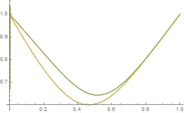
 Plot[
   {eps1, eps2, eps3}, {p2, 0, 1}, PlotRange -> {{0, 1}, {0.4, 1}}, 
   PlotLegends -> "Expressions", GridLines -> Automatic
 ]

The problem is that this is a small example, but I have to do this several times for bigger matrices. Is there a way to plot the outputs in a more efficient manner?

score 2 · Accepted Answer · answered Mar 05 '19 at 17:05

Note that your replacement in the definition of sol does not work as you wrote it; since you have p1 in the first replacement rule, you either chain the two rules (i.e. /. p3 -> 1 - p1 - p2 /. p1 -> 0, or you use ReplaceRepeated (//.) with the list.

You then can use a replacement within Plot to get what you want no matter how many solutions you seek. Note that you want to Evaluate the argument of Plot so that Plot can realize that it is a list and color your curves appropriately:

det2 = -λ^3 - λ^2*(p1 + p2) + λ*(p1 - p2)^2 + p3^3 + (p1 - p2)^2*(p1 + p2)
sol = Solve[det2 == 0, λ] //. {p3 -> 1 - p1 - p2, p1 -> 0}

Plot[Evaluate[Abs@λ /. sol], {p2, 0, 1}]

Mathematica graphics

(The need for Evaluate stems from the HoldAll attribute of Plot, see Plot draws list of curves in same color when not using Evaluate.

score 1 · Answer 2 · edited Mar 05 '19 at 16:47

1

Try

sol = Solve[det2 == 0, λ] /. p3 -> 1 - p1 - p2 /. p1 -> 0
Plot[
  λ /. sol, {p2, 0, 1}, PlotRange -> {{0, 1}, {0.4, 1}}, 
  PlotLegends -> "Expressions", GridLines -> Automatic]

Only one solution is plotted because some complex λ

edited Mar 05 '19 at 16:47

MarcoB

67,153
18
91
189

answered Mar 05 '19 at 14:19

Ulrich Neumann

53,729
2
23
55

Thank you. Yes, I forgot to take the absolute value in the code. – mors Mar 05 '19 at 14:35

score 1 · Answer 3 · answered Mar 05 '19 at 14:35

1

Try this one,

eps1 = sol[[1, All]];

eps2 = sol[[2, All]];

eps3 = sol[[3, All]];

Plot[Evaluate@ReIm@{eps1, eps2, eps3} /. {p1 -> 0}, {p2, 0.01, 1}, PlotRange -> All]

answered Mar 05 '19 at 14:35

zhk

11,939
1
22
38

Thanks, but for some reason, I could not be able to make the plot, I ended with an empty plot. At the end, to make the plot I used eps=sol[[All, 1, 2]] and eps[[1]], eps[[2]], eps[[3]]; I have to admit that I am still trying to understand the syntax. – mors Mar 05 '19 at 15:33

Plotting Solve output automatically

3 Answers3