Generating FittedModels from vector-valued linear model fits

Question

I have vector-valued data with normally distributed noise that I want to analyse. Assumptions on data can be made; in this specific example, it's expected that components of fitted vector values always have a unit sum.

Here's a toy example of manually finding a fit with these constraints:

With[{source = {x^2 / 2, 1 - x^2 / 2 - x, x}},
 With[{
   coeff = {a, b, c, d, e, f},
   eqn =
    {a x^2 + b x + c, d x^2 + e x + f, 
     1 - (a x^2 + b x + c) - (d x^2 + e x + f)},
   data = 
    Table[{x, 
      source + RandomVariate[NormalDistribution[0, .1], 3]}, {x, 0, 1, .025}]},
  Sum[SquaredEuclideanDistance[v[[2]], eqn /. x -> v[[1]]], {v, data}] //
     eqn /. Last@Minimize[# /. Abs -> Identity, coeff, Reals] & // Echo //
   Show[
    ListPlot[
     Transpose[{{#1, #2[[1]]}, {#1, #2[[2]]}, {#1, #2[[3]]}} & @@@ data]],
    Plot[Join[source, #], {x, 0, 1}, Evaluated -> True]] &]]

{-0.0162628+0.0842304 x+0.43683 x^2,0.99686 -0.908144 x-0.608563 x^2,0.0194033 +0.823914 x+0.171733 x^2}

Now I have a curve fit for each vector component, but what I would really want is corresponding FittedModel objects with "MeanPredictionBands" and such properties. Is there any way to cross this gap, practically creating a model with the above fitting polynomial as "BestFit"?

EDIT: Looking at InputForm of FittedModel objects would suggest this is feasible. Most of the arguments seem straight-forward, although some on the end of the definition are not that obvious.

Possible duplicate: https://mathematica.stackexchange.com/questions/87927/fit-model-with-two-dependent-variables. — JimB, Mar 09 '19 at 15:15
The potential downside to the possible duplicate is that one would need to be able to assume that the error variances are the same for all 3 equations. If that's not a feasible assumption for real-world data, then using LogLikelihood and FindMaximum functions would allow for potentially unequal variances. — JimB, Mar 09 '19 at 15:21
The answer I gave below is wrong if the triplets of observations sum exactly to 1 as opposed to just the expected values summing to one. If the former, then by definition the 3 observations are correlated with each other and that doesn't yet seem to be addressed by either of the two current answers. (The estimates of the coefficients won't change much - if at all - but the estimates of the standard errors of the coefficients and the predictions will be off. — JimB, Mar 11 '19 at 01:44

JimB · Accepted Answer · 2019-03-11T00:04:48.447

While you know how to put this altogether from scratch, I suspect that some will not be able to construct the confidence or prediction bands reliably in such a manner. If it is a reasonable assumption that the error variances are the same for all models, then just modifying the input data is about all that's necessary to get the desired output from NonlinearModelFit. (I make too many mistakes so I need to go that route.)

First, include in some dummy variables in the data:

(* Sample data using dummy variables:
1,0,0 => data from model 1
0,1,0 => data from model 2
0,0,1 => data from model 3 *)
data={{1, 0, 0, 0., -0.0988754}, {0, 1, 0, 0., 0.936639}, {0, 0, 1, 0., -0.168444}, {1, 0, 0, 0.025, -0.0201999}, {0, 1, 0, 0.025, 1.02862}, {0, 0, 1, 0.025, -0.0562009}, {1, 0, 0, 0.05, -0.0120367}, {0, 1, 0, 0.05, 0.870238}, {0, 0, 1, 0.05, -0.0936423}, {1, 0, 0, 0.075, -0.128804}, {0, 1, 0, 0.075, 0.985538}, {0, 0, 1, 0.075, 0.125768}, {1, 0, 0, 0.1, 0.078006}, {0, 1, 0, 0.1, 0.775311}, {0, 0, 1, 0.1, 0.0928273}, {1, 0, 0, 0.125, 0.121525}, {0, 1, 0, 0.125, 0.71475}, {0, 0, 1, 0.125, 0.0477607}, {1, 0, 0, 0.15, 0.115014}, {0, 1, 0, 0.15, 0.851672}, {0, 0, 1, 0.15, 0.0933949}, {1, 0, 0, 0.175, -0.0260633}, {0, 1, 0, 0.175, 0.721085}, {0, 0, 1, 0.175, 0.2533}, {1, 0, 0, 0.2, 0.0929319}, {0, 1, 0, 0.2, 0.741054}, {0, 0, 1, 0.2, 0.246308}, {1, 0, 0, 0.225, -0.121485}, {0, 1, 0, 0.225, 0.558944}, {0, 0, 1, 0.225, 0.180121}, {1, 0, 0, 0.25, 0.196925}, {0, 1, 0, 0.25, 0.739204}, {0, 0, 1, 0.25, 0.216802}, {1, 0, 0, 0.275, 0.00288085}, {0, 1, 0, 0.275, 0.531013}, {0, 0, 1, 0.275, 0.364702}, {1, 0, 0, 0.3, -0.0748257}, {0, 1, 0, 0.3, 0.452435}, {0, 0, 1, 0.3, 0.246644}, {1, 0, 0, 0.325, -0.102033}, {0, 1, 0, 0.325, 0.552273}, {0, 0, 1, 0.325, 0.307822}, {1, 0, 0, 0.35, 0.012419}, {0, 1, 0, 0.35, 0.493619}, {0, 0, 1, 0.35, 0.109975}, {1, 0, 0, 0.375, 0.174347}, {0, 1, 0, 0.375, 0.403849}, {0, 0, 1, 0.375, 0.640423}, {1, 0, 0, 0.4, 0.0267628}, {0, 1, 0, 0.4, 0.50906}, {0, 0, 1, 0.4, 0.249802}, {1, 0, 0, 0.425, 0.145036}, {0, 1, 0, 0.425, 0.401913}, {0, 0, 1, 0.425, 0.365026}, {1, 0, 0, 0.45, 0.0917381}, {0, 1, 0, 0.45, 0.452611}, {0, 0, 1, 0.45, 0.191856}, {1, 0, 0, 0.475, 0.05115}, {0, 1, 0, 0.475, 0.461663}, {0, 0, 1, 0.475, 0.370011}, {1, 0, 0, 0.5, 0.275475}, {0, 1, 0, 0.5, 0.20153}, {0, 0, 1, 0.5, 0.479379}, {1, 0, 0, 0.525, 0.184857}, {0, 1, 0, 0.525, 0.26697}, {0, 0, 1, 0.525, 0.586871}, {1, 0, 0, 0.55, 0.236133}, {0, 1, 0, 0.55, 0.379411}, {0, 0, 1, 0.55, 0.61064}, {1, 0, 0, 0.575, 0.241561}, {0, 1, 0, 0.575, 0.243509}, {0, 0, 1, 0.575, 0.508213}, {1, 0, 0, 0.6, 0.220454}, {0, 1, 0, 0.6, 0.118133}, {0, 0, 1, 0.6, 0.595092}, {1, 0, 0, 0.625, 0.12719}, {0, 1, 0, 0.625, 0.126479}, {0, 0, 1, 0.625, 0.644849}, {1, 0, 0, 0.65, 0.114451}, {0, 1, 0, 0.65, 0.144761}, {0, 0, 1, 0.65, 0.581061}, {1, 0, 0, 0.675, 0.197143}, {0, 1, 0, 0.675, 0.186537}, {0, 0, 1, 0.675, 0.705692}, {1, 0, 0, 0.7, 0.231923}, {0, 1, 0, 0.7, -0.0542245}, {0, 0, 1, 0.7, 0.939961}, {1, 0, 0, 0.725, 0.318287}, {0, 1, 0, 0.725, 0.0657639}, {0, 0, 1, 0.725, 0.609313}, {1, 0, 0, 0.75, 0.177536}, {0, 1, 0, 0.75, 0.0269016}, {0, 0, 1, 0.75, 0.741112}, {1, 0, 0, 0.775, 0.357059}, {0, 1, 0, 0.775, -0.191036}, {0, 0, 1, 0.775, 0.830267}, {1, 0, 0, 0.8, 0.188352}, {0, 1, 0, 0.8, -0.0579005}, {0, 0, 1, 0.8, 0.695232}, {1, 0, 0, 0.825, 0.271996}, {0, 1, 0, 0.825, -0.304167}, {0, 0, 1, 0.825, 0.832492}, {1, 0, 0, 0.85, 0.408437}, {0, 1, 0, 0.85, -0.0930686}, {0, 0, 1, 0.85, 0.717563}, {1, 0, 0, 0.875, 0.570663}, {0, 1, 0, 0.875, -0.286103}, {0, 0, 1, 0.875, 0.96456}, {1, 0, 0, 0.9, 0.340535}, {0, 1, 0, 0.9, -0.25579}, {0, 0, 1, 0.9, 0.672478}, {1, 0, 0, 0.925, 0.0811443}, {0, 1, 0, 0.925, -0.332707}, {0, 0, 1, 0.925, 0.841893}, {1, 0, 0, 0.95, 0.327199}, {0, 1, 0, 0.95, -0.43617}, {0, 0, 1, 0.95, 0.849182}, {1, 0, 0, 0.975, 0.359762}, {0, 1, 0, 0.975, -0.67714}, {0, 0, 1, 0.975, 0.950295}, {1, 0, 0, 1., 0.494625}, {0, 1, 0, 1., -0.533217}, {0, 0, 1, 1., 1.09384}};

(* Define equation using dummy variables *)
eqn[m1_, m2_, m3_, x_, a_, b_, c_, d_, e_, f_] :=
 {m1, m2, m3}.{a x^2 + b x + c, d x^2 + e x + f, 
   1 - (a x^2 + b x + c) - (d x^2 + e x + f)}

(* Run regression *)
coeff = {a, b, c, d, e, f};
nlm = NonlinearModelFit[data, eqn[m1, m2, m3, x, a, b, c, d, e, f], 
   coeff, {m1, m2, m3, x}];

(* Get mean prediction bands *)
mpb1 = nlm["MeanPredictionBands"] /. {m1 -> 1, m2 -> 0, m3 -> 0};
mpb2 = nlm["MeanPredictionBands"] /. {m1 -> 0, m2 -> 1, m3 -> 0};
mpb3 = nlm["MeanPredictionBands"] /. {m1 -> 0, m2 -> 0, m3 -> 1};

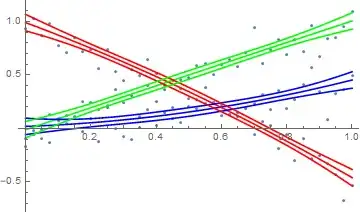
(* Show data, fit, and mean prediction bands *)
Show[ListPlot[data[[All, {4, 5}]]],
 Plot[{nlm[1, 0, 0, x], nlm[0, 1, 0, x], nlm[0, 0, 1, x]}, {x, 0, 1},
  PlotStyle -> {Blue, Red, Green}],
 Plot[{mpb1, mpb2, mpb3}, {x, 0, 1},
  PlotStyle -> {Blue, Blue, Red, Red, Green, Green}]]

And this works even if the model is not a polynomial.

kirma · Answer 2 · 2019-03-11T05:39:53.477

I dug a bit into FittedModel and it would seem pretty straight-forward to reconstruct FittedModels for simple linear model fits of one-dimensional data. As a result, I created a PreFittedLinearModel function which takes data, fitted polynomial (plus options, such as Weights) as input, and returns a FittedModel object as a result:

ClearAll@PreFittedLinearModel;

Options[PreFittedLinearModel] = 
  FilterRules[Options[LinearModelFit], 
   ConfidenceLevel | Tolerance | VarianceEstimatorFunction | Weights |
     WorkingPrecision];

PreFittedLinearModel[data_, poly_, var_, OptionsPattern[]] :=
 With[{funs = Table[var^i, {i, 0, Exponent[poly, var]}]},
  FittedModel @@ {
    {"Linear", N@CoefficientList[poly, var], {{var}, funs}, {0, 0}},
    {N[OptionValue[Weights] /. Automatic -> Table[1, Length@data]]}, 
    data, Table[N@funs, {var, data[[All, 1]]}], 
    Function[Null, Internal`LocalizedBlock[{var}, #], {HoldAll}], 
    Sequence @@ (# -> OptionValue[#] & /@ {ConfidenceLevel, Tolerance,
         VarianceEstimatorFunction, WorkingPrecision})}]

Now I can check how (95%) confidence intervals compare with my original function:

With[{source = {x^2/2, 1 - x^2/2 - x, x}},
 With[{
    coeff = {a, b, c, d, e, f},
    eqn = {
      a x^2 + b x + c, d x^2 + e x + f, 
      1 - (a x^2 + b x + c) - (d x^2 + e x + f)},
    data = 
     Table[{x, 
       source + RandomVariate[NormalDistribution[0, .1], 3]}, {x, 0, 1, .025}]},
   Sum[SquaredEuclideanDistance[v[[2]], eqn /. x -> v[[1]]], {v, data}] //
     eqn /. Last@Minimize[# /. Abs -> Identity, coeff, Reals] & //
     PreFittedLinearModel[{#1, #2[[3]]} & @@@ data, #[[3]], x] &] //
   Plot[Join[{x}, #["MeanPredictionBands"]], {x, 0, 1}, 
    Evaluated -> True] &]

... but, as @JimB stated, this approach has issues in its core.

EDIT: Probably I should modify this to work with any linear combination of functions, and extract polynomial coefficient functions for this generalized version instead of assuming a polynomial. Polynomials just happened to be the tool I used originally...

Generating FittedModels from vector-valued linear model fits

2 Answers2