I don't think transforming the non-autonomous system into that autonomous system is the right way to go. Notice that the equilibria you mention both have {y, z} == {0, 0}, which contradicts the given periodic forcing.
Instead, I suggest transforming it by adding $dt/dt=1$ (see e.g. Strogatz 2015, p. 8). Plotting that vector field using myStreamPlot (original by @Rahul) from here:
sp = myStreamPlot[{1, (2 + Cos[2 π t]) x - 0.5 x^2 - 0.5},
  {t, 0, 4}, {x, -10, 10}, AspectRatio -> 0.3, ImageSize -> 600,
  FrameLabel -> {"t", "x"}]
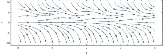
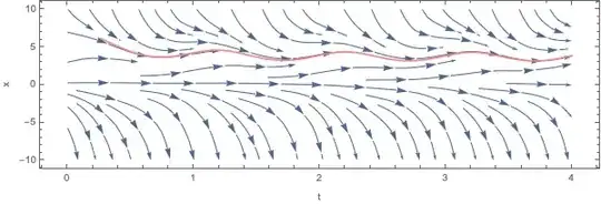
You can already make out a stable limit cycle oscillating around $x \approx 4$, but to highlight it with a trajectory from NDSolve:
sol = NDSolve[{x'[t] == (2 + Cos[2 π t]) x[t] - 0.5 x[t]^2 - 0.5,
  x[0] == 8}, x, {t, 0, 4}][[1]];
Show[sp, Plot[x[t] /. sol, {t, 0, 4}, PlotStyle -> Pink]]
Reference:
Strogatz SH. 2015. Nonlinear Dynamics and Chaos: With Applications to Physics, Biology, Chemistry, and Engineering. 2nd ed.
x~0.27– Ulrich Neumann Jul 23 '19 at 10:440.27and it is unstable. But I'm more familiar with the phase diagram with Axesxandx', and the stable limit cycle will converge to a closed curve. Is it possible to plot in this way within the vector field? – keanhy14 Jul 23 '19 at 11:16x''. Only thing I can think of is wrapping it around a cylinder as done here but I don't think that will be particularly insightful. – Chris K Jul 23 '19 at 11:44