How to implement a Kalman or LQG regulator in the control of classical pendulum problem

Question

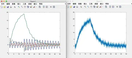
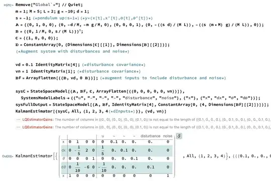
My final purpose is to realize an LQG control of inverted pendulum.

To this end, my first step I think is to build a Kalman regulator in Mathematica. The original Matlab version of Kalman filter is written by Steve Brunton. I try to follow his code, but I am stuck when using the Mathematica command KalmanEstimator which complains “The number of columns in * is not equal to the length of * ”.

Any suggestions will be greatly appreciated.

Thanks.

My Mathematica code is below.

Remove["Global`*"] // Quiet;

m = 1;
M = 5;
L = 2;
g = -10;
d = 1;

s = -1; (* pendulum up: s=1 *)

(* y={x[t], x'[t], \[Theta][t], \[Theta]'[t]} *)
\[DoubleStruckCapitalA] = {{0, 1, 0, 0}, {0 , -d/M, -m g/M, 0}, {0, 0,0, 1}, {0, - ((s d )/(M L)), -((s (m + M) g)/(M L)), 0}};
\[DoubleStruckCapitalB] = {{0, 1/M, 0, s/(M L)}}\[Transpose];
\[DoubleStruckCapitalC] = {{1, 0, 0, 0}};
\[DoubleStruckCapitalD] = ConstantArray[0, {Dimensions[\[DoubleStruckCapitalC]][[1]], Dimensions[\[DoubleStruckCapitalB]][[2]]}];


(*Augment system with disturbances and noise*)
vd = 0.1  IdentityMatrix[4]; (* disturbance covariance *)
vn = 1 IdentityMatrix[1];(*disturbance covariance*)

(* augment inputs to include disturbance and noise *)
\[DoubleStruckCapitalB]F = ArrayFlatten[{{\[DoubleStruckCapitalB], vd, 0 \[DoubleStruckCapitalB]}}]; 
sysC = StateSpaceModel[{\[DoubleStruckCapitalA], \[DoubleStruckCapitalB]F, \[DoubleStruckCapitalC], ArrayFlatten[{{0, 0, 0, 0, 0, vn}}]},
SystemsModelLabels -> {{"u", "-", "-", "-", "disturbance", "noise"}, {"x"}, {"x", "dx", "\[Theta]", "d\[Theta]"}}]
sysFullOutput = StateSpaceModel[{\[DoubleStruckCapitalA], \[DoubleStruckCapitalB]F, IdentityMatrix[4], ConstantArray[0, {4, Dimensions[\[DoubleStruckCapitalB]F][[2]]}]}];

KalmanEstimator[{sysC, All, {1, 2, 3, 4(*dInputs*)}}, {vd, vn}]

Maybe the matlab code and its result is helpful, so I also pasted them here.

clear all, close all, clc
m = 1;
M = 5;
L = 2;
g = -10;
d = 1;
s = -1; % pendulum up (s=1)
% y = [x; dx; theta; dtheta];
A = [0 1 0 0;
    0 -d/M -m*g/M 0;
    0 0 0 1;
    0 -s*d/(M*L) -s*(m+M)*g/(M*L) 0];
B = [0; 1/M; 0; s*1/(M*L)];
C = [1 0 0 0];  
D = zeros(size(C,1),size(B,2));
%%  Augment system with disturbances and noise
Vd = .1*eye(4);  % disturbance covariance
Vn = 1;       % noise covariance
BF = [B Vd 0*B];  % augment inputs to include disturbance and noise
sysC = ss(A,BF,C,[0 0 0 0 0 Vn]);  % build big state space system... with single output
sysFullOutput = ss(A,BF,eye(4),zeros(4,size(BF,2)));  % system with full state output, disturbance, no noise
%%  Build Kalman filter
[L,P,E] = lqe(A,Vd,C,Vd,Vn);  % design Kalman filter
Kf = (lqr(A',C',Vd,Vn))';   % alternatively, possible to design using "LQR" code
sysKF = ss(A-L*C,[B L],eye(4),0*[B L]);  % Kalman filter estimator
%%  Estimate linearized system in "down" position (Gantry crane)
dt = .01;
t = dt:dt:50;
uDIST = randn(4,size(t,2));
uNOISE = randn(size(t));
u = 0*t;
u(100:120) = 100;     % impulse
u(1500:1520) = -100;  % impulse
uAUG = [u; Vd*Vd*uDIST; uNOISE];
[y,t] = lsim(sysC,uAUG,t);
[xtrue,t] = lsim(sysFullOutput,uAUG,t);
[x,t] = lsim(sysKF,[u; y'],t);
plot(t,xtrue,'-',t,x,'--','LineWidth',2)
figure
plot(t,y)
hold on
plot(t,xtrue(:,1),'r')
plot(t,x(:,1),'k--')

------------------------------- Updated post:-------------------------

1. including a sinusoidal input
2. setting up an LQG based feedback control

Updated questions:

@Suba Thomas, thanks for your answer :) It is really, really helpful. I still have some questions.

1. You seems delete the measurement noise from the input. Is it possible to include the stochastic measurements noise in the input (of system sysC), just like what Matlab did ?

2. With the help of your code, I try to include (1) a sinusoidal input and (2) to setup an LQG based feedback control. I updated my post to include the code for these two attempts. Am I doing correctly in these two efforts?

3. I am teaching myself some optimal control theory. However, I found that there are some confusing differences between contents of books and Mathematica. For example, few books mentioned descriptor state-space model, few books distinguish deterministic, feedback, stochastic inputs. Can you recommend a book that more close to Mathematica?

   Thanks.

Updated code:

Remove["Global`*"] // Quiet;

m = 1;
M = 5;
L = 2;
g = -10;
d = 1;
s = -1; \[DoubleStruckCapitalA] = {{0, 1, 0, 0}, {0, -d/M, -m g/M, 
   0}, {0, 0, 0, 1}, {0, -((s d)/(M L)), -((s (m + M) g)/(M L)), 0}};
\[DoubleStruckCapitalB] = {{0, 1/M, 0, s/(M L)}}\[Transpose];
\[DoubleStruckCapitalC] = {{1, 0, 0, 0}};
\[DoubleStruckCapitalD] = {{0, 0, 0, 0, 0, 0.1}};
vd = 0.1 IdentityMatrix[4];
vn = 1 IdentityMatrix[1];

bs = {{1, 0, 0, 
    0}}\[Transpose];(* postion vector for the \
determinstic(sinusoidal) input (usin) *)
\[DoubleStruckCapitalB]F = 
 ArrayFlatten[{{\[DoubleStruckCapitalB], vd, bs}}];

sysC = StateSpaceModel[{\[DoubleStruckCapitalA], \
\[DoubleStruckCapitalB]F, \[DoubleStruckCapitalC], \
\[DoubleStruckCapitalD]}, 
   SystemsModelLabels -> {{"u", "d1", "d2", "d3", "d4", 
      "usin"}, {"x"}, {"x", "dx", "\[Theta]", "d\[Theta]"}}];

q = 10 IdentityMatrix[4]; r = 0.1 IdentityMatrix[1];
(* lqg regulator *)

lqg = LQGRegulator[{sysC, All, {1}, {6}}, {vd, vn}, {q, r}];

sscl = SystemsModelStateFeedbackConnect[sysC, lqg, {1}, {1}];

y = OutputResponse[{sscl, {1, 0, 0, 0, 0, 0, 0, 0}}, {Sin[t]}, {t, 0, 
    50}];
Plot[y, {t, 0, 50}, PlotRange -> All]

Answer 1

The system sysC needs to be modified as

\[DoubleStruckCapitalB]F = ArrayFlatten[{{\[DoubleStruckCapitalB], vd}}];

sysC = StateSpaceModel[{\[DoubleStruckCapitalA], \
\[DoubleStruckCapitalB]F, \[DoubleStruckCapitalC]}, 
  SystemsModelLabels -> {{"u", "d1", "d2", "d3", "d4"}, {"x"}, {"x", 
 "dx", "\[Theta]", "d\[Theta]"}}]

Then the Kalman estimator can be constructed as

sysKF = SystemsModelExtract[KalmanEstimator[{sysC, All, 1}, {vd, vn}], All, -1]

Trying to replicate the inputs used in the Matlab code.

range = Range[0, 50, 0.1];

impulseInput = 100 (UnitStep[t - 1] - UnitStep[t - 1.2] - 
   UnitStep[t - 20] + UnitStep[t - 20.22]);

processNoise = Table[Interpolation[
 Thread[{range, 
   RandomReal[
    NormalDistribution[0, Sqrt[0.1]], {Length@range}]}]][t + 0.1], 4];

measurementNoise = Interpolation[
 Thread[{range, 
  RandomReal[NormalDistribution[0, 1], {Length@range}]}]][t + 0.1];

The actual, true, or noisy outputs of the system.

xtrue = OutputResponse[sysFullOutput, Flatten@{impulseInput, processNoise}, {t, 0, 49}];
xtrue[[1]] += measurementNoise;
Plot[xtrue, {t, 0, 49}, PlotRange -> All]

Compute the filtered response and compare it to the actual.

OutputResponse[sysKF, Flatten@{impulseInput, xtrue[[1]]}, {t, 0, 49}];
Plot[{xtrue[[1]], %}, {t, 0, 49}, PlotRange -> All, PlotLegends -> {"Actual", "Filtered"}]

Followup to the updated question

For simulation, you can use sysCwith the measurement noise included as in the Matlab code. However even the Matlab function lqe does not use that sysC for computing the gains. It is a rather wearisome design for these functions like KalmanEstimator etc to have a system with the matrices for the measurement noise included because it involves appending the system with zero matrices. Also, this noise is better characterized as noisy measurements and not as noisy inputs. With the latter, we have to distinguish between two kinds of noisy inputs - one affecting the process and the other the measurement. As things stand, there are two options: a) Create sysCwith the measurement noise included, and delete them when passing it to KalmanEstimator and avoid using AddTo during simulation. b) Create sysC without the measurement noise, compute the gains with KalmanEstiamtor and then use AddTo during simulation.

You need to use SystemsModelFeedbackConnect, and not SystemsModelStateFeedbackConnect. Also it does not make sense to have $sin(t)$ as an input. It is a regulator and not tracker, and the natural reference input of the former is 0. If you want $x$ to track a reference $ x_{ref} $ add an additional state $x_i=\int(x_{ref}-x) dt$. Regulating that along with the others will try to drive $x$ to $x_{ref}$. If you are designing for a specific reference signal then you can try AsymptoticOutputTracker.

The function design is based on the standard control configuration [wikipedia]. The books on that page are all excellent ones. Descriptor systems are a bit different. Some of the equations we had to derive and make sure. But for the most part they are based on the book by Guang-Ren Duan [Springer].