Solving for a minimum action path in mathematica

Question

I am interested in computing a quantity that is mathematically defined as follows,

$$\phi(x_1,x_2) = \inf_{T>0} \inf_{\gamma \in C^{x_2}_{x_1 }(0,T)} \int_{0}^T L(\gamma, \dot{\gamma})\mathrm{d}t$$

where $x_1,x_2$ are points in $\mathbb{R}^n$ and $C^{x_2}_{x_1 }(0,T) = \{ \gamma: [0,T]\rightarrow \mathbb{R}^n| \gamma(0) = x_1, \gamma(T) = x_2 \}$ is the set of curves joining the two points $x_1, x_2$. $T$ represents, a time coordinate and the integrand is a an action $S$ with the corresponding Lagrangian. I am interested in paths which minimise the action, connecting $x_1, x_2$, and computing $\phi$ along those paths.

Supposing I know the Hamiltonian, one way I could think of doing this is writing the action in terms of: $S = \int_{0}^{t} \sum_i p_i\dot{q_i}-H(p,q)$, since essentially I am interested in curves in phase space that join two points and are parametrised by $T$, and minimise the action functional, they must satisfy Hamiltonian equations of motion (if I understand my mechanics correctly).

To solve the Hamiltonian equations of motion: $$\dot{q_i} = \partial_{p_i} H(p,q)$$ $$\dot{p_i} = -\partial_{q_i} H(p,q)$$

However, instead of initial conditions, I would like to specify a boundary value problem, $q(0) = q_1, q(T) = q_2, p(0) = p_1, p(0) = p_2$.

For this purpose I tried using NDSolve. Given a Hamiltonian, (j = 60, here $\rho,r$ stand in for $q, p$ respectively.

h2[j, \[Rho], 
  r] := ((-(1/900))*(-1 + 
      E^r)*(\[Rho]*(7921 + 7021*(-2 + \[Rho])*\[Rho]) + 
          E^r*(-1 + \[Rho])*(900 + 7021*\[Rho]^2)))/E^r



\[Rho]dt[j, \[Rho], 
  r] := ((1/900)*(\[Rho]*(-7921 - 7021*(-2 + \[Rho])*\[Rho]) - 
      E^(2*r)*(-1 + \[Rho])*(900 + 7021*\[Rho]^2)))/E^r

rdt[j, \[Rho], 
  r] := ((1/900)*(-1 + E^r)*(7921 + 7021*\[Rho]*(-4 + 3*\[Rho]) + 
      E^r*(900 + 7021*\[Rho]*(-2 + 3*\[Rho]))))/E^r

sp = StreamPlot[{rdt[j, \[Rho], r], \[Rho]dt[j, \[Rho], r]}, {r, -0.1,
    2}, {\[Rho], 0., 1}, StreamColorFunction -> "Purple", 
  PlotRange -> Full]

cp = ContourPlot[{rdt[j, \[Rho], r], \[Rho]dt[j, \[Rho], 
    r]}, {r, -0.1, 2}, {\[Rho], 0., 1}]
pp = ParametricPlot[{Log[(\[Rho] (-7921 - 
       7021 (-2 + \[Rho]) \[Rho]))/((-1 + \[Rho]) (900 + 
       7021 \[Rho]^2))], \[Rho]}, {\[Rho], 0, 1}, 
  PlotStyle -> {Thick, Red}]

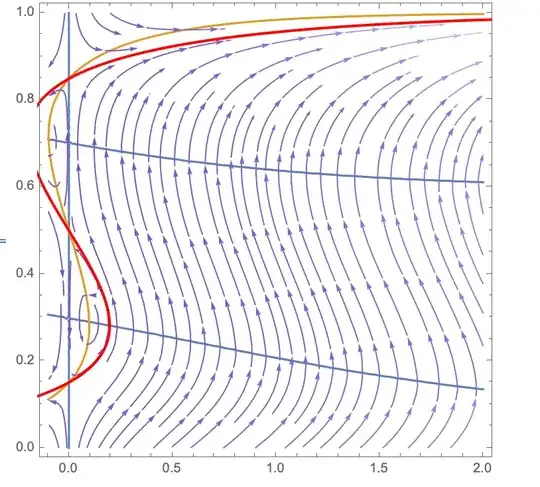
Here, I have plotted the stream and contour plots for the two equations, along with the zero energy (H=0) contour. I would expect the minimum action plot between the the two fixed points, 0.15 and 0.5 ought to lie on the zero energy contour.

Now, I deploy NDSolve, following @Michael E2's second suggestion. (Choosing T to be sufficiently large, because techincally the transition is only possible in infinite T.

sols = FullSimplify[NDSolve[{D[[Rho][t], t] == D[h2[j, [Rho][t], r[t]], r[t]], D[r[t], t] == -D[h2[j, [Rho][t], r[t]], [Rho][t]], [Rho][0] == 0.151, [Rho][10^4] == 0.5}, {[Rho][t], r[t]}, {t, 0, 10^4}]]

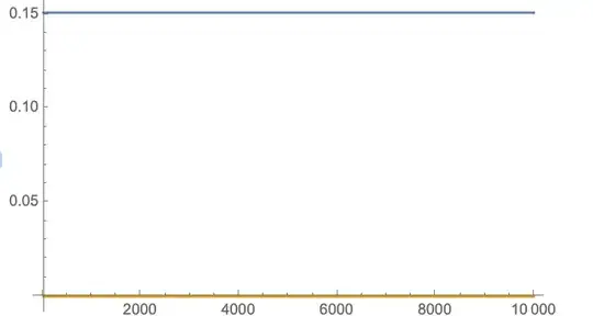
Plotting the interpolating functions,

not quite what i wanted.

Outside of this particular example, is there built in functionality to find paths that minimize action in Mathematica, that can work for arbitrary systems in $\mathbb{R^n}$?

EDIT: It was recommended that I add some context to the problem. These types of optimisations appear in the context of stochastic dynamics and large deviation theory, and the quantity $\phi$ is the Friedlin-Wentzel quasipotential.