A suitable strategy to estimate numerically a complex integral. How to use "MaxErrorIncreases"?

Question

I am trying to numerically estimate a complex 3D integral. Here is its version considerably reduced for the purposes of the present discussion:

NIntegrate[(x + ξ)^4/(
 Sqrt[ξ] (y^2 + (x + ξ)^2)^3), {x, -100, 100}, {y, 0, 
  100}, {ξ, 0, 100}]

The integral has an integrable singularity. One can make it sure by passing to spherical coordinates. I believe that it should be possible to calculate it. However, it is this singularity that makes the integral difficult to estimate numerically. Regularization like

...{y, 0.001,100}, {ξ, 0.001, 100}...

does not help.

I tried most (though yet not all) of methods and strategies for the singular integrals listed in the tutorial/NIntegrateIntegrationStrategies. This was so far unsuccessful.

One of the recommendations I received in the message reporting the divergence was to increase "MaxErrorIncreases". However, I failed to find any documentation showing how to apply this option. Therefore,

My first question: Do you know, how to use "MaxErrorIncreases"?

The second question: Do you have any idea on calculating an integral of this type?

Edit: To address the question of @Akku14 Yes, I managed to integrate it over ksi exactly:

intt = Integrate[
  1/Sqrt[ξ]* ((x + ξ)^4)/(y^2 + (x + ξ)^2)^3, {ξ, 
   0, ∞}, Assumptions -> {y > 0, x ∈ Reals}]

which yields

(* 1/64 π (10 (1/(x - I y)^(3/2) + 1/(x + I y)^(3/2)) - (
   12 I (1/Sqrt[x - I y] - 1/Sqrt[x + I y]))/y + 
   3 I (1/(x - I y)^(5/2) - 1/(x + I y)^(5/2)) y)  *)

On the one hand, this result seems suspicious. I am not quite sure that it is right. On the other hand, this does not really help. The integral

NIntegrate[intt, {x, -100, 100}, {y, 0, 100}]

still does not converge, at least, by itself.

@yarchik No. The actual integrand has also a step-like function as a factor. The latter is zero beyond +-100 along x, +100 along y and ksi. This makes the limits finite. I omitted this factor, since the difficulty is related to the singularity, rather than to this factor, and it will make the question more obscure. On the other hand, like this, the limits given above are to extent arbitrary. One can instead +-100 take +-10 to try. — Alexei Boulbitch, Mar 02 '20 at 09:50
The shown example is analytically integrable with respect to at least one variable. May be your real problem is also integrable with Integrate in x,y or xi. This makes things much easier. — Akku14, Mar 02 '20 at 10:35
You could also play with the singularity handler. Usage example: Method -> {"GlobalAdaptive", "SingularityHandler" -> "DuffyCoordinates", "SingularityDepth" -> 20, "MaxErrorIncreases" -> 20000}. See http://reference.wolfram.com/language/tutorial/NIntegrateIntegrationStrategies.html for documentation of these options. Good luck. Nothing really worked for me yet. — Michael E2, Mar 02 '20 at 13:31
@Michael E2 Thank you, I will try. MaxErrorIncreases is a part of my question. Why do not you formulate your comment as an answer? — Alexei Boulbitch, Mar 02 '20 at 13:40
For me the principal problem is calculating the integral, which I've failed to do, almost as bad as entering MaxErrorIncreases into the documentation search bar. My goodness, not a single relevant hit until the 17th (NIntegrate), which is the only relevant hit in all 33 hits. The tutorial I linked does not even come up in the whole list. Your first question should have been "easily found in the documentation," but it's not. — Michael E2, Mar 02 '20 at 13:59
Here is a discussion of MaxErrorIncreases I wrote up for another question, but I didn't get a chance to post it: the question was closed before I got a chance. https://gist.github.com/mroge02/a2d99912f5f885b5d2e9e28281272b71 — Michael E2, Mar 06 '20 at 02:04
@Michael E2 Thank you very much. It is very informative, and I learned it with a great pleasure. Thank you once more. The errors visualization I find especially useful. Strange that such a function has not been implemented as a standard. — Alexei Boulbitch, Mar 06 '20 at 10:04
The discussion of MaxErrorIncreases is now on-site here: https://mathematica.stackexchange.com/a/215891/4999 — Michael E2, Mar 06 '20 at 22:23
@Michael E2 Michael, could you please kindly let me know what error estimates the function errorPlot? Is it the absolute error or the relative one? I thank you once more for this function, which is very helpful. — Alexei Boulbitch, Mar 13 '20 at 14:33
Relative error. The absolute error is gathered with IntegrationMonitor :> (Sow[Total@Through[#@"Error"]] &)]. This is converted to relative error with errors = Flatten@errors/integral;, the RealExponent of which is what is plotted. For a near-zero integral, the absolute error is probably more appropriate; one could change the line to errors = Flatten@errors. (Probably the original should be divided by Abs[integral], but RealExponent doesn't care if the numbers are negative or even complex.) -- Glad you find it helpful. Thanks! — Michael E2, Mar 13 '20 at 15:08

score 1 · Answer 1 · answered Mar 03 '20 at 14:00

At present I developed a workaround for this problem. It is lengthily, and, generally, I do not like it very much. However, it seems to work. I will be grateful for all sorts of criticisms and suggestions.

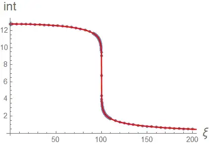
So, let us first integrate over x and y, and find out this integral as the function of ξ. Note that I make a regularization of the denominator by the machine number 10^-16.

    iter = Join[Table[10^-i, {i, 0, 16}] // N, Table[i, {i, 2, 90, 5}], 
    Table[i, {i, 91, 110, 0.1}], Table[i, {i, 115, 200, 5}]] // Sort;

Here iter is a non-homogeneous iterator.

Below int is the list of values of pairs {ξ, integralOverXandY}

int = Table[{ξ, 
        NIntegrate[(x + ξ)^4/( (y^2 + (x + ξ)^2)^3 + 
          10^-16), {x, -100, 100}, {y, 0, 100}, 
         Method -> {"LocalAdaptive", 
           Method -> {"ClenshawCurtisRule", "Points" -> 10}}, 
         AccuracyGoal -> 3, PrecisionGoal -> 5]}, {ξ, iter}];

In the following I interpolate the results:

f = Interpolation[int, InterpolationOrder -> 1];
Show[{
  ListPlot[int, PlotRange -> All, 
   AxesLabel -> {Style["ξ", 16], Style["int", 16]}],
  Plot[f[ξ], {ξ, 0.0001, 300}, PlotStyle -> Red]
  }]

It looks as follows:

Now it can be integrated over ξ:

NIntegrate[f[ξ]/Sqrt[ξ], {ξ, 10^-16, 300}]

(*  261.063   *)

I also tried to calculate the integral over x and y with the options:

Method -> {"AdaptiveMonteCarlo", "MaxPoints" -> 1000000}, 
 AccuracyGoal -> 2, PrecisionGoal -> 4]

and

Method -> {"GlobalAdaptive", Method -> "GaussKronrodRule"}, 
 AccuracyGoal -> 2, PrecisionGoal -> 4]

This returns error messages but makes the calculation. The plot appears considerably worse, but the result of integration is astonishingly the same.

With the help of Rubi I could integrate first over y and then over x analytically, The result has a removable singularity, where you have a jump. But the function looks quite different. This 1D function can then be integrated numerically. — yarchik, Mar 04 '20 at 21:46
@yarchik Thank you. It is a very valuable observation. I will try it up. My preliminary trial shows that the result of the Rubi integration over x and y does not coincide with my numeric result, neither does it with my expectation (the latter, of course, may be wrong). I will look at it precisely. Why do not you write your comment as an answer? — Alexei Boulbitch, Mar 05 '20 at 10:24

score 0 · Answer 2 · answered Mar 03 '20 at 14:57

(Extended comment...)

It might be a good idea to run NIntegrate computational set-up with a few different option settings in order to verify the integral values. For example,

AbsoluteTiming[
 Association@
  Table[i -> 
    NIntegrate[(x + \[Xi])^4/(Sqrt[\[Xi]] (y^2 + (x + \[Xi])^2)^3), {x, -100, 100}, {y, 0, 100}, {\[Xi], 0, 100}, MinRecursion -> i, 
     MaxRecursion -> 100, 
     Method -> {"LocalAdaptive", "SymbolicProcessing" -> 0, 
       "SingularityHandler" -> None, 
       Method -> {"ClenshawCurtisRule", "Points" -> 10}}, 
     AccuracyGoal -> 3, PrecisionGoal -> 5], {i, 1, 10}]
 ]

(* {72.8907, <|1 -> 142.097, 2 -> 158.287, 3 -> 174.651, 
  4 -> 174.651, 5 -> 174.651, 6 -> 174.651, 7 -> 174.651, 
  8 -> 174.651, 9 -> 174.651, 10 -> 174.651|>} *)

Thank you I am going to do this. If you have in mind some options that are more promising then others, I would be grateful to know it. — Alexei Boulbitch, Mar 03 '20 at 15:03

A suitable strategy to estimate numerically a complex integral. How to use "MaxErrorIncreases"?

2 Answers2

Linked