Is it possible to use `ContourPlot` for specific eigenvalue of a large matrix Mn(x,y)?

Question

I have a large matrix, say En En, as a function of two variables x and y which has En eigenvalues. I want to use ContourPlot to show specific eigenvalue, say (En/2)+1 with respect to x and y. For small En this can be done but it did not work for large En. For example, with En=8 it gives the desired result, but for larger En not working.

M1={{0, I Sin[x] + Sin[y], 3 - Cos[x] - Cos[y], -1}, {-I Sin[x] + Sin[y],
   0, -1, 3 - Cos[x] - Cos[y]}, {3 - Cos[x] - Cos[y], -1, 
  0, -I Sin[x] - Sin[y]}, {-1, 3 - Cos[x] - Cos[y], I Sin[x] - Sin[y],
   0}};

tc={{0, 0, 0, 0}, {0, 0, 0, 0}, {-1, 0, 0, 0}, {0, -1, 0, 0}};

Mn[n_] := 
 SparseArray[{Band[{1, 1}, {4 n, 4 n}] -> {M1}, 
   Band[{1, 5}, {4 n, 4 n}] -> {tc}, 
   Band[{5, 1}, {4 n, 4 n}] -> {ConjugateTranspose[tc]}}]

 w = 2; En = 4 w;(*w must be >1*)
ContourPlot[
 Evaluate[Eigenvalues[N@Mn[w]][[En/2 + 1]] == 0.4], {x, -2, 
  2}, {y, -2, 2}, ContourShading -> None, ContourStyle -> Blue]

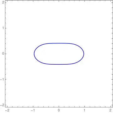
this is the result with w=2 (i.e En=8) How can I do the same for w=40 (En=160)?

I try w=3 and got this error "Eigenvalues::eival: Unable to find all roots of the characteristic polynomial." and this is the final output:

Answer 1

There is no need to calculate the eigenvalues explicitly; it is enough to check that the characteristic polynomial has a zero. If you calculate the determinant numerically for specific numerical values of $x$, $y$, and the eigenvalue, then the characteristic polynomial can be circumvented and more stable algorithms can be applied:

MM[x_, y_] = Mn[w];
f[λ_?NumericQ, {x_?NumericQ, y_?NumericQ}] := 
  Det[MM[x, y] - λ*IdentityMatrix[En]]

With[{λ = 0.4}, 
  ContourPlot[f[λ, {x, y}] == 0, {x, -2, 2}, {y, -2, 2}]]

Alternatively, use the trick of this solution: for given $(x,y)$, calculate the eigenvalue that is closest to $\lambda$ by using a shifted Arnoldi-Lanczos iteration, and then contour-plot the difference between this eigenvalue and $\lambda$. This method is much faster and much more stable, but generates spurious contours whenever there's a switch from one eigenvalue branch to another:

g[λ_?NumericQ, {x_?NumericQ, y_?NumericQ}] := 
  Eigenvalues[MM[x, y], 1, 
              Method -> {"Arnoldi", "Criteria" -> "Magnitude", 
                         "Shift" -> λ}][[1]] - λ

With[{λ = 0.4}, 
  ContourPlot[g[λ, {x, y}] == 0, {x, -2, 2}, {y, -2, 2}]]