Mathematica will not solve this numerical equation

Question

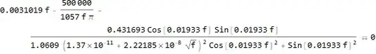
I have the following equation:

eq = 0.003101895368576676` f - 500000/(1057 f \[Pi]) - (0.43169299511061626` Cos[0.019329990640367303` f] Sin[0.019329990640367303` f])/(1.0609` (1.37`*^-11 + 0.222185005727138`*^-7 Sqrt[f])^2 Cos[0.019329990640367303` f]^2 + Sin[0.019329990640367303` f]^2) == 0

Mathematica does not seem to be able to solve it for any of it's roots, f.

NSolve[eq, f]

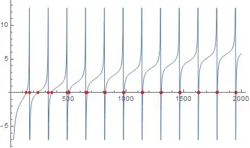
Just returns the input. Same with Solve[]. However, I can plot the left hand side without any problems:

Plot[(eq // First) /. f -> freq, {freq, 20, 2000}]

So how come Mathematica can't find any numerical solutions?

As mentioned in the Details section of document of NSolve: NSolve deals primarily with linear and polynomial equations. So it's not surprising to find it fail on transcendental equation. You may want to read this: https://mathematica.stackexchange.com/q/91784/1871 — xzczd, Apr 10 '20 at 05:11

Nasser · Accepted Answer · 2020-04-10T07:17:10.617

9

ClearAll[f]
eq = 0.003101895368576676` f - 
   500000/(1057 f \[Pi]) - (0.43169299511061626` Cos[
       0.019329990640367303` f] Sin[
       0.019329990640367303` f])/(1.0609` (1.37`*^-11 + 
          0.222185005727138`*^-7 Sqrt[f])^2 Cos[
         0.019329990640367303` f]^2 + 
      Sin[0.019329990640367303` f]^2) == 0

Mathematica graphics

 sol = NSolve[{eq && 20 < f < 2000}, f]

Mathematica graphics

p1 = Plot[eq, {f, 20, 2000}];
pts = Table[{f /. sol[[j]], eq[[1]] /. sol[[j]]}, {j, 1, Length[sol]}];

Mathematica graphics

p2 = ListPlot[pts, PlotStyle -> Red];
Show[p1, p2]

Mathematica graphics

edited Apr 10 '20 at 07:17

answered Apr 10 '20 at 05:26

Nasser

143,286
11
154
359

Ah, restricting the domain for f did it, thanks Nasser. – Jeremiah Rose Apr 10 '20 at 05:57
In retrospect, it was very stupid of me to expect NSolve to give me an answer for an infinitely periodic function without defining a domain. – Jeremiah Rose Apr 10 '20 at 06:03
2

@Nasser, you may not count the singularities as zeros. Test it with Table[eq[[1]] /. sol[[j]], {j, 1, Length[sol]}] which shows {3.33067*10^-16, -0.000569916, 2.22045*10^-16, 0.000642054, -1.11022*10^-16, 0.0000471086, 6.66134*10^-16, 0.00181685, 3.9968*10^-15, 0.000928914, 2.66454*10^-15, 0.000213413, 2.66454*10^-14, 0.00217025, 1.9984*10^-14, -0.000959413, 1.04361*10^-13, 0.000527678, 6.83897*10^-14, -0.000158866, -5.68434*10^-14, -0.000788316, 2.39808*10^-14, 0.000126493, 8.88178*10^-15} . – Akku14 Apr 10 '20 at 06:07
@Akku14 you are right, I was lazy did not check, but it was good approximation :). It should be OK now. Thanks. – Nasser Apr 10 '20 at 07:17

bill s · Answer 2 · 2020-04-10T22:48:20.363

You are looking for the root of the function:

x[f_] := 0.003101895368576676` f - 500000/(1057 f \[Pi]) - (0.43169299511061626` Cos[0.019329990640367303` f] Sin[0.019329990640367303` f])/(1.0609` (1.37`*^-11 + 0.222185005727138`*^-7 Sqrt[f])^2 Cos[0.019329990640367303` f]^2 + Sin[0.019329990640367303` f]^2);

FindRoot has no trouble:

FindRoot[x[f] == 0, {f, 1}]
{f -> 134.145}

You can find the other roots by giving more or different starting values:

roots = FindRoot[x[f] == 0, {f, Range[1, 1000, 10]}];
f /. roots // Union

{134.145, 134.145, 234.019, 354.49, 504.565, 504.565, 662.105, 821.956, 982.803, 982.803}

Mathematica will not solve this numerical equation

2 Answers2