Define a color function using Piecewise

Question

How can I define a ColorFunction for my ContourPlot using Piecewise? For example, after making a ContourPlot for this function:

p[x_, y_] := 1 - Sin[x]^2 Sin[y]^2;

I want to define my ColorFunction in a way that for example for 0 < p < 0.1 the plot have a different color than 0.1 < p < 0.2. An example of what I need is in the following plot: my example

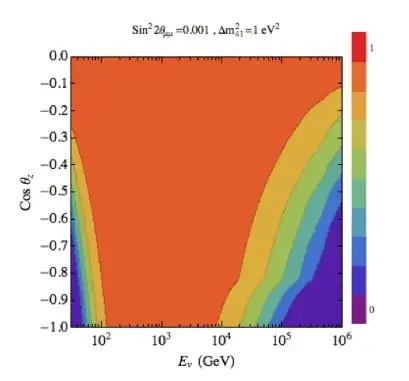
where the colorbar at the right shows that each color corresponds to a value of p.

Doesn't it just work by default? ContourPlot[1 - Sin[x]^2*Sin[y]^2, {x, 0, Pi}, {y, 0, Pi}, PlotLegends -> Automatic, ColorFunction -> "DarkRainbow"] — Vitaliy Kaurov, Mar 25 '13 at 23:00
@VitaliyKaurov Kaurov The thing is that I need to have control on the colors. In the plot that I have put as an example, e.g. dark orange corresponds to 0.8<p<0.9. ColorFunction -> "DarkRainbow" doesn't give me this option. — tenure track job seeker, Mar 25 '13 at 23:03

score 8 · Accepted Answer · edited Jun 19 '13 at 13:43

myBlend[x_] := Blend[{Purple, Blue, Cyan, Green, Yellow, Orange, Red}, x]
ContourPlot[p[x, y], {x, 0, \[Pi]}, {y, 0, \[Pi]}, 
 Contours -> 25, ColorFunction -> myBlend]

or

myPiecewise[x_] := Piecewise[{{Red, 0 <= x <= 0.25}, 
  {Orange, 0.25 < x <= 0.75}, {Yellow, 0.75 < x <= 1}]
ContourPlot[p[x, y], {x, 0, \[Pi]}, {y, 0, \[Pi]}, 
  ColorFunction -> myPiecewise, ColorFunctionScaling -> False]

Remember to put ColorFunctionScaling -> False if you need precise control over the position of the colours.

<< PlotLegends`
ShowLegend[
  ContourPlot[2 p[x, y], {x, 0, \[Pi]}, {y, 0, \[Pi]}, 
     ColorFunction -> myPiecewise],
  {myPiecewise, 10, "0", "1", LegendPosition -> {1.1, 0}}]

guide/PlotLegendsPackage

Note: I work with version 8. In version 9 it appears to have been integrated: ref/BarLegend

Thanks a lot for your help. Do you know how can I build that color column at the right hand side of the plot in the question? I need to explain the colors using that. — tenure track job seeker, Mar 25 '13 at 23:12

score 4 · Answer 2 · answered Jun 19 '13 at 15:46

There's another syntax for Blend which lets you control the color-banding easily:

cf = Blend[{
    {0., Blue}, 
    {0.1, Green},
    {0.15, Black},
    {0.2, Red}, 
    {0.8, Purple},
    {0.95, Cyan}
    }, #1] & 

 DensityPlot[Sin[a] Sin[b],
   {a, -2 Pi, 2 Pi}, 
   {b, -2 Pi, 2 Pi}, 
   PlotPoints -> 250,
   ColorFunction -> cf ,
   MaxRecursion -> 2,
   ColorFunctionScaling -> False,
   ImageSize -> 500]

color function and densityplot

Define a color function using Piecewise

2 Answers2

Linked