FEM stress analysis by considering thermal strain

Question

Following the question in this post, I am trying to do a stress analysis by including thermal strain. @user21 already showed how to do a pre-stressed analysis. Analogically, I modified the code and included a thermal strain term. Let's consider a very simple case that the thermal strain [Epsilon]t is uniform in the body.

\[Epsilon]t = 0.0001.
pst = {Inactive[
Div][{{-(Y/(1 - \[Nu]^2)), 
0}, {0, -((Y*(1 - \[Nu]))/(2*(1 - \[Nu]^2)))}} . 
Inactive[Plus][
Inactive[Grad][u[x, y], {x, y}], {\[Epsilon]t, 0}], {x, y}] + 
Inactive[
Div][{{0, -((Y*\[Nu])/(1 - \[Nu]^2))}, {-((Y*(1 - \[Nu]))/(2*(1 \- \[Nu]^2))), 0}} . 
Inactive[Plus][
Inactive[Grad][v[x, y], {x, y}], {0, \[Epsilon]t}], {x, y}], 
Inactive[
Div][{{0, -((Y*(1 - \[Nu]))/(2*(1 - \[Nu]^2)))}, \
{-((Y*\[Nu])/(1 - \[Nu]^2)), 0}} . 
Inactive[Plus][
Inactive[Grad][u[x, y], {x, y}], {\[Epsilon]t, 0}], {x, y}] + 
Inactive[
Div][{{-((Y*(1 - \[Nu]))/(2*(1 - \[Nu]^2))), 
0}, {0, -(Y/(1 - \[Nu]^2))}} . 
Inactive[Plus][
Inactive[Grad][v[x, y], {x, y}], {0, \[Epsilon]t}], {x, y}]};

Let's consider the same geometry, but with the beam bottom and left surfaces restrained and no external forces applied:

Needs["NDSolve`FEM`"];
L = 1;
h = 0.125;
reg = Rectangle[{0, -h}, {L, h}];
mesh = ToElementMesh[reg];
materialParameters = {Y -> 10^3, \[Nu] -> 33/100};

{uif, vif} = 
NDSolveValue[{pst == {0, 0}, 
DirichletCondition[u[x, y] == 0, x == 0], 
DirichletCondition[v[x, y] == 0, y == -h]} /. 
materialParameters, {u, v}, {x, y} \[Element] mesh];

dmesh = ElementMeshDeformation[mesh, {uif, vif}, "ScalingFactor" -> 1];
Show[{mesh["Wireframe"], 
dmesh["Wireframe"[
"ElementMeshDirective" -> Directive[EdgeForm[Red], FaceForm[]]]]}]

I think the problem is straightforward, but I cannot make this code run. Can anybody help?

Where you got the system of equations? Usually the thermal stress is defined as a volumetric force proportional to $\nabla T$. — Alex Trounev, May 03 '20 at 09:08
@AlexTrounev, thank you! Sorry, I am new to FEM stress analysis. Can you please further explain why we should use et=T0 (x+y) ? I actually need to do an analysis with nonuniform thermal strain in the body, so your explain would help me solve my final problem — XIJUN SHI, May 03 '20 at 18:24
We can use any function et[x,y]. I used linear function as an example. Practically we should include equation for temperature in the system and solve it together with elasticity equations. — Alex Trounev, May 03 '20 at 18:52
@AlexTrounev Thanks. How about modeling a uniform thermal strain for verification purpose? A uniform thermal strain in the body can be et=T0, right? Then this becomes my original code. However, the displacements are 0 if I use et=T0, which does not make sense (there should be displacements). — XIJUN SHI, May 03 '20 at 19:11
We have et under Div[] operator. So with et=T0 we have zero effect. Linear function it is the simplest case of thermal effect. Also we can put this on a border as a DirichletCondition[] or NeumannValue[]. But you put both zero. So what effect you expect? — Alex Trounev, May 03 '20 at 19:29
@AlexTrounev, thank you Alex for your patiently answering my questions. I am still a new learner so I probably lack fundamental understanding of the system equation. I put pst=={0,0} because this is a traction free body (only thermal effect is considered, no other external or body forces). What is the physical meaning of your example et=T0 (x+y) when T0=1/10? Does this represent that the entire body is subjected to a uniform thermal strain of 0.1? — XIJUN SHI, May 03 '20 at 19:48
@AlexTrounev My thought process was that I need to add a free strain term (which is the thermal strain) to the mechanical strain (Grad[u[x.y]] and Grad[v[x.y]]), so I came up with the system equation. Probably the system equation was wrong at the first place. — XIJUN SHI, May 03 '20 at 19:50
No, the system of equation is not wrong and it could be compare with a standard notation using $\nabla T$. If we put et=T0 f[x,y] then $T0 \nabla f/(1+\nu)=\alpha \nabla T$, thus $f=\alpha (1+\nu) T/T0$. It demonstrates that thermal effect could be only with non zero temperature gradient. — Alex Trounev, May 03 '20 at 20:42

score 8 · Answer 1 · answered May 03 '20 at 10:00

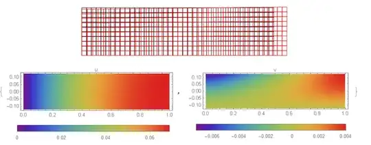
We have replaced $\epsilon t\rightarrow et, \nu\rightarrow nu$ and put et=T0 (x+y). Also we used Activate in NDSolve. Code:

et = T0 (x + y);
pst = {Inactive[
      Div][{{-(Y/(1 - nu^2)), 
        0}, {0, -((Y*(1 - nu))/(2*(1 - nu^2)))}}.Inactive[Plus][
       Inactive[Grad][u[x, y], {x, y}], {et, 0}], {x, y}] + 
    Inactive[
      Div][{{0, -((Y*nu)/(1 - 
             nu^2))}, {-((Y*(1 - nu))/(2*(1 - nu^2))), 0}}.Inactive[
        Plus][Inactive[Grad][v[x, y], {x, y}], {0, et}], {x, y}], 
   Inactive[
      Div][{{0, -((Y*(1 - nu))/(2*(1 - nu^2)))}, {-((Y*nu)/(1 - 
             nu^2)), 0}}.Inactive[Plus][
       Inactive[Grad][u[x, y], {x, y}], {et, 0}], {x, y}] + 
    Inactive[
      Div][{{-((Y*(1 - nu))/(2*(1 - nu^2))), 
        0}, {0, -(Y/(1 - nu^2))}}.Inactive[Plus][
       Inactive[Grad][v[x, y], {x, y}], {0, et}], {x, y}]};


Needs["NDSolve`FEM`"];
L = 1;
h = 0.125;
reg = Rectangle[{0, -h}, {L, h}];
mesh = ToElementMesh[reg];
materialParameters = {Y -> 10^3, nu -> 33/100, T0 -> 1/10};


{uif, vif} = 
  NDSolveValue[{Activate[pst == {0, 0} /. materialParameters], 
    DirichletCondition[u[x, y] == 0, x == 0], 
    DirichletCondition[v[x, y] == 0, y == -h]}, {u, 
    v}, {x, y} \[Element] mesh];

Visualisation

dmesh = ElementMeshDeformation[mesh, {uif, vif}, "ScalingFactor" -> 1];
Show[{mesh["Wireframe"], 
  dmesh["Wireframe"[
    "ElementMeshDirective" -> Directive[EdgeForm[Red], FaceForm[]]]]}]

{DensityPlot[uif[x, y], {x, y} \[Element] mesh, 
  ColorFunction -> "Rainbow", 
  PlotLegends -> Placed[Automatic, Bottom], PlotLabel -> "u", 
  AspectRatio -> Automatic], 
 DensityPlot[vif[x, y], {x, y} \[Element] mesh, 
  ColorFunction -> "Rainbow", 
  PlotLegends -> Placed[Automatic, Bottom], PlotLabel -> "v", 
  AspectRatio -> Automatic]}

score 6 · Answer 2 · answered May 04 '20 at 05:11

6

There is a PDE model collection in the documentation. Among other examples there is a Thermal Load on a Beam application example. You can base your work off of that.

answered May 04 '20 at 05:11

user21

39,710
8
110
167

thank you! Very useful! – XIJUN SHI May 04 '20 at 06:48

score 1 · Answer 3 · answered Sep 21 '21 at 14:16

I have also been struggling to understand the implementation of thermal strains, and here is an alternative attempt that may also help others. These strains are essentially the same as "eigenstrains" or "stress-free" strains. The idea being that an element without constraint will have a certain strain due to swelling, thermal expansion/contraction, phase transformation etc. It is still unclear to me whether it is possible to directly compute the role of thermal strains (like @Alex Trounev) has done, or whether one needs to use a time dependent model. As @XIJUN SHI suggested in the comments simulations of a uniform thermal strain (i.e. a mono material with a constant temperature) should be possible, however if one does this by for example inserting et = T0 ; in @Alex Trounev's code, as this is a constant it disappears and the final strain/deformation is zero.

@Alex Trounev suggested coupling this with a model for temperature changes. We can do this by using some of the code from the Thermal Load on a Beam example mentioned by @user21. The idea is to have a temperature load that is time dependent, and we include this as a body force and solve as a function of time.

To keep the code consistent we use the same as above:

Needs["NDSolve`FEM`"];
L = 1;
h = 0.125;
reg = Rectangle[{0, -h}, {L, h}];
mesh = ToElementMesh[reg];
materialParameters = {Y -> 10^3, nu -> 33/100, \[Rho] -> 0.001, \[Alpha] -> 0.001};

Rho is a density term , alpha is our thermal expansion coefficient.

We define a stress operator the same as done in the example

pst={\[Rho] D[u[t,x,y],{t,2}]+
Inactive[Div][{{-(Y/(1 - nu^2)), 0}, {0, -((Y*(1 - nu))/(2*(1 - nu^2)))}} . Inactive[Grad][u[t, x, y], {x, y}], {x, y}] + 
 Inactive[Div][{{0, -((Y*nu)/(1 - nu^2))}, {-((Y*(1 - nu))/(2*(1 - nu^2))), 0}} . Inactive[Grad][v[t, x, y], {x, y}], {x, y}],
\[Rho] D[v[t,x,y],{t,2}]+Inactive[Div][{{0, -((Y*(1 - nu))/(2*(1 - nu^2)))}, {-((Y*nu)/(1 - nu^2)), 0}} . Inactive[Grad][u[t, x, y], {x, y}], {x,y}] + Inactive[Div][{{-((Y*(1 - nu))/(2*(1 - nu^2))), 0}, {0, -(Y/(1 - nu^2))}} .Inactive[Grad][v[t, x, y], {x, y}], {x, y}]} /.materialParameters;

We define a temperature function that goes from T = 0 to T = 1 and is uniform over the mesh.

Tfun[t, x, y] = t;

We now introduce the thermal load as a body force.

fx = Inactive[Div][{-(Y \[Alpha]/(1 - nu)) Tfun[t, x, y], 0}, {x, y}] /.materialParameters;
fy = Inactive[Div][{0, -(Y \[Alpha]/(1 - nu)) Tfun[t, x, y]}, {x, y}] /. materialParameters;

Add in boundary conditions and initial conditions:

gd = {DirichletCondition[{u[t, x, y] == 0., v[t, x, y] == 0.}, x == 0 && y == 0], DirichletCondition[{u[t, x, y] == 0.}, x == 0]};
ic = {u[0, x, y] == 0, v[0, x, y] == 0, (D[u[t, x, y], t] == 0) /. t -> 0, (D[v[t, x, y], t] == 0) /. t -> 0};
pde = {pst == {fx, fy}, gd, ic};

We can now solve:

{uif, vif} = NDSolveValue[pde, {u, v}, {t, 0, 1}, {x, y} \[Element] mesh];

and plot now the strain in the x-direction

Plot[D[uif[1, x, 0.0], x] // Evaluate, {x, 0, 1},PlotRange -> {{0, 1.1}, {0, 0.002}}]

The strain is now 0.001, (same as the thermal strain). A similar graph is achieved for the strain in the y-direction.

I hope this is helpful.

FEM stress analysis by considering thermal strain

3 Answers3

Linked