Irregular Confluent Hypergeometric Functions (Spherical Coulomb Wavefunctions)

Question

I want to program in the regular and irregular spherical Coulomb wavefunctions $F_\ell(\gamma,kr)$ and $G_\ell(\gamma,kr)$, respectively, which are defined in terms of the regular and irregular solutions to Kummer's differential equation

$$\Big[z\frac{d^2}{dz^2}+(\beta-z)\frac{d}{dz}-\alpha\Big]\,f(z)=0\,.$$

The regular solution is given by the standard confluent hypergeometric function ${}_1F_1(\alpha;\,\beta;\,z)$. I can access this function in Mathematica using Hypergeometric1F1, out of which I can construct the regular spherical Coulomb wavefunction $F_\ell(\gamma,kr)$.

But I am unable to find the two irregular solutions, typically denoted $W_1$ and $W_2$. I need these to construct the irregular spherical Coulomb wavefunction. The $W$'s and the regular ${}_1F_1$ are connected by the relations:

$${}_1F_1(\alpha|\,\beta|\,z)=W_1(\alpha|\,\beta|\,z)+W_2(\alpha|\,\beta|\,z)$$

Does anyone know how I can access both irregular solutions?

Answer 1

EDIT

The functions CoulombF[], CoulombG[], CoulombH1[], and CoulombH2[] are now built-in, starting from version 13.

---

Old version

The formulae here also allow for an expression in terms of the irregular Whittaker function WhittakerW[]:

CoulombPhase[ℓ_, η_] := (LogGamma[1 + ℓ + I η] - LogGamma[1 + ℓ - I η])/(2 I)
CoulombHPlus[ℓ, η, ρ_] :=
             Exp[π (η - I ℓ)/2 + I CoulombPhase[ℓ, η]] WhittakerW[-I η, ℓ + 1/2, -2 I ρ]
CoulombHMinus[ℓ, η, ρ_] :=
              Exp[π (η + I ℓ)/2 - I CoulombPhase[ℓ, η]] WhittakerW[I η, ℓ + 1/2, 2 I ρ]

Compare with OP's implementation (which has a different argument convention):

N[{CoulombHPlus[2/3, 3/4, 5], CoulombHplus[2/3, 4/3, 5 3/4]}]
   {-0.93049 + 0.597603 I, -0.93049 + 0.597603 I}
N[{CoulombHMinus[2/3, 3/4, 5], CoulombHminus[2/3, 4/3, 5 3/4]}]
   {-0.93049 - 0.597603 I, -0.93049 - 0.597603 I}

These are of course the complex-valued solutions (they are related to the real solutions in a way similar to the relationship of the Hankel functions with the Bessel functions); if one wants the real-valued irregular solution, this is easily done. For completeness, I will also include an implementation of the regular Coulomb function:

CoulombFactor[ℓ_, η_] :=
      Exp[-π (η + I (ℓ + 1))/2] Sqrt[Gamma[1 + ℓ - I η] Gamma[1 + ℓ + I η]]/(2 (2 ℓ + 1)!)
CoulombF[ℓ, η, ρ_] := CoulombFactor[ℓ, η] WhittakerM[I η, ℓ + 1/2, 2 I ρ]
CoulombG[ℓ, η, ρ_] := (CoulombHPlus[ℓ, η, ρ] + CoulombHMinus[ℓ, η, ρ])/2

Compare:

N[{(CoulombHPlus[2/3, 3/4, 5] - CoulombHMinus[2/3, 3/4, 5])/(2 I),
   CoulombF[2/3, 3/4, 5]}] // Chop
   {0.597603, 0.597603}
N[{(CoulombHPlus[2/3, 3/4, 5] + CoulombHMinus[2/3, 3/4, 5])/2,
   CoulombG[2/3, 3/4, 5]}] // Chop
   {-0.93049, -0.93049}

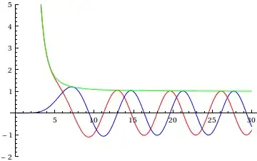
Replicate the plots here:

With[{ℓ = 0, η = Sqrt[15/2]}, 
     Plot[{CoulombF[ℓ, η, ρ], CoulombG[ℓ, η, ρ], Abs[CoulombHPlus[ℓ, η, ρ]]}, {ρ, 0, 30}, 
          PlotRange -> {-2, 5}, PlotStyle -> {Blue, Red, Green}]]

With[{ℓ = 5, η = 0}, 
     Plot[{CoulombF[ℓ, η, ρ], CoulombG[ℓ, η, ρ], Abs[CoulombHPlus[ℓ, η, ρ]]}, {ρ, 0, 30}, 
          PlotRange -> {-2, 5}, PlotStyle -> {Blue, Red, Green}]]

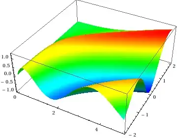
and the plots here:

(* from http://dlmf.nist.gov/help/vrml/aboutcolor;
   cf. https://mathematica.stackexchange.com/a/101933 *)
DLMFHeightColor = Hue[2 (1 - #)/3] &;
Plot3D[CoulombF[0, η, ρ], {ρ, 0, 5}, {η, -2, 2}, BoundaryStyle -> None,
       ColorFunction -> DLMFHeightColor, Mesh -> False, PlotPoints -> 75,
       WorkingPrecision -> 20]

Plot3D[CoulombG[0, η, ρ], {ρ, 0, 5}, {η, -2, 2}, BoundaryStyle -> None,
       ClippingStyle -> None, ColorFunction -> DLMFHeightColor,
       Mesh -> False, PlotPoints -> 55, WorkingPrecision -> 20]

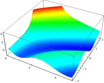
I needed to use arbitrary precision evaluation for these plots since the evaluation of the Coulomb functions with these definitions at machine precision seemed unstable for some combinations of arguments (try them yourself). There should be a way to reformulate these formulae for better stability (there are already a number of papers on the numerical evaluation of Coulomb functions), but I don't have time to look through those at the moment.

Answer 2

I stumbled upon the NIST Digital Library of Mathematical Functions online, and the relations given in section 33.2 are sufficient to program the useful Coulomb wavefunctions into Mathematica. My implementation is as follows:

The Sommerfeld parameter:

γ[k_] = 1/k

The irregular Coulomb functions $H^{\pm}_\ell(\gamma,\,kr)$

coulθ = (k r - γ[k] Log[2 k r] - ℓ π/2 + Arg[Gamma[ℓ + 1 + I γ[k]]]);

CoulombHplus[ℓ_, k_, r_] = E^(I coulθ) (-2 I k r)^(ℓ + 1 + I γ[k])
   HypergeometricU[ℓ + 1 + I γ[k],  2 ℓ + 2, -2 I k r];
CoulombHminus[ℓ_, k_, r_] = E^(-I coulθ) (2 I k r)^(ℓ + 1 - I γ[k])
   HypergeometricU[ℓ + 1 - I γ[k], 2 ℓ + 2, 2 I k r];

Then the standard regular and irregular Coulomb functions follow: $F_\ell(\gamma,\,kr)$ and $G_\ell(\gamma,\,kr)$

CoulombF[ℓ_, k_, r_] = 1/(2 I) (CoulombHplus[ℓ, k, r] - CoulombHminus[ℓ, k, r]);
CoulombG[ℓ_, k_, r_] = 1/2 (CoulombHplus[ℓ, k, r] + CoulombHminus[ℓ, k, r]);

A good consistency check is to compare against their known asymptotic behavior as $r\to\infty$:

asympCoulombF[ℓ_, k_, r_] =
     Sin[k r - π ℓ/2 - γ[k] Log[2 k r] + Arg[Gamma[ℓ + 1 + I γ[k]]]];
asympCoulombG[ℓ_, k_, r_] =
     Cos[k r - π ℓ/2 - γ[k] Log[2 k r] + Arg[Gamma[ℓ + 1 + I γ[k]]]];