How can I superimpose a set of points on a ContourPlot?

Question

I am familiar with Mathematica to a certain extent, but its subtleties still elude me.

Currently I am trying to solve the following problem:
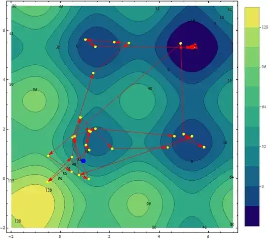
The function $f(x,y)$ is continuous. I know how to create a contourplot of it. I also have a list of points {{x,y}, ...} which I would like to insert into my contour plot.

Background:
I am working on some genetic algorithms and would like to visualize how the population converges to the global optimum. This is why I would like to show the population (or at least the best candidate of each generation) in the contour plot.

How could this be done?

A contour plot is 2D. How do you want to include 3D points in it? — Dr. belisarius, Mar 29 '13 at 11:26
contour plot projects onto the x-y plane the levels of a function in two variables. It is 2D as opposed to your triples. You could project them too using ListContourPlot or use a the contour plot as a texture for the x-y plane (see related) — gpap, Mar 29 '13 at 11:31
i did not mean to use 3D data - my question was perhaps somewhat confusion. Just wanted to plot the population - only (x,y) values. I will adjust the phrasing accordingly — Probabilitnator, Mar 29 '13 at 11:56

score 12 · Accepted Answer · edited Apr 13 '17 at 12:55

12

I guess one should use the following plot to visualize convergence. For optimization consider this example, and collect the points during NMinimize evaluation.

Clear[f]
f[x_, y_] := 20 Sin[\[Pi]/2 (x - 2 \[Pi])] +
20 Sin[\[Pi]/2 (y - 2 \[Pi])] + (x - 2 \[Pi])^2 + (y - 2 \[Pi])^2;
pts = Reap[sol = NMinimize[f[x, y], {x, y}, 
  Method -> {"SimulatedAnnealing", "PerturbationScale" -> 3, 
    "BoltzmannExponent" -> 
     Function[{i, df, f0}, -df/(Exp[i/10])]}, 
  StepMonitor :> (Sow[{x, y}])];];

Let's visualize it. Here blue is the starting point and red is the global optimum.

ContourPlot[f[x, y], {x, -2, 7}, {y, -2, 7}, Contours -> 10, 
ColorFunction -> "BlueGreenYellow", PlotLegends -> Automatic, 
Epilog -> ({Red, PointSize[.01], Arrowheads[0.025], 
Arrow /@ Partition[pts[[2, 1]], 2, 1], Yellow, 
Point /@ pts[[2, 1]], Blue, PointSize[.02], Point[pts[[2, 1, 1]]],
 Red, PointSize[.02], Point[{x, y} /. sol[[2]]]}),ContourLabels -> True]

enter image description here

Note:

For plotting 3D points on a 2D surface, check out this wonderful post by Rahul Narain.

BR

edited Apr 13 '17 at 12:55

Community

1

answered Mar 29 '13 at 11:43

PlatoManiac

14,723
2
42
74

this is beautiful. Problem is I wrote my own genetic algorithm in C++ and output the different evolutionary steps into a CSV-file. This is why I need to plot a list of data. – Probabilitnator Mar 29 '13 at 11:59
still i had no idea sth like that wos doable. Beautiful :) – Probabilitnator Mar 29 '13 at 12:03
@Probabilitnator please note pts are just the points visited by the algorithm. So what you need to do is import the points of your genetic steps into Mathematica. CSV import is easy. – PlatoManiac Mar 29 '13 at 12:05
now i see. Thanks now this is even more beautiful <3 ! – Probabilitnator Mar 29 '13 at 12:13
is this Rastrigin's function you are using - this is actually the one I wanted to do the plot for :D – Probabilitnator Mar 29 '13 at 12:14
1

@chris mostly copied from docs :( Thx though.... – PlatoManiac Mar 29 '13 at 21:20

score 2 · Answer 2 · answered Mar 29 '13 at 11:33

2

Since presumably f[x,y] is the same for the GA result as the contour plot, you can display the points at which your GA has been evaluated on the contour plot in this way:

gaPoints= Tuples[Range@12, 2];
f[{x_, y_}] := {Sin@x, Cos@y}

g1 = ListPlot[gaPoints];
g2 = ContourPlot[f[{x, y}], {x, 0, 4 Pi}, {y, 0, 4 Pi}];

And plot the two graphs as:

Show[g2, g1]

Mathematica graphics

answered Mar 29 '13 at 11:33

image_doctor

10,234
23
40

so basically I am just overlapping the two plots ?? - this is easier than I would have thought and exactly what I am looking for. Could you perhaps explain some of the syntax ? (why use 'Sin@x' ) – Probabilitnator Mar 29 '13 at 12:02
Yes indeed you can combine plots by simply overlapping them :) Sin@x is just a short form of Sin[x]. – image_doctor Mar 29 '13 at 15:00
how can I get rid of that grid ? – Probabilitnator Mar 29 '13 at 16:39
1

You can use the ContourLines Options, ContourPlot[f[{x, y}], {x, 0, 4 Pi}, {y, 0, 4 Pi}, ContourLines -> False] – image_doctor Mar 29 '13 at 23:21

How can I superimpose a set of points on a ContourPlot?

2 Answers2

Linked

Related