What is the most accurate way of getting the highest derivative from NDSolve?

Question

I would like to compare my simulations in Mathematica to measured data. I measure acceleration but for simulations the starting point is displacement. How does one get accurate simulations of higher derivatives of the solutions to differential equations?

Here is a simple example of a simulation where we have the exact solution. (My actual problems are much more complicated). First I define a few parameters and then get exact results for displacement, velocity and acceleration.

vals = {
   a -> 100, (* frequency *)
   b -> 10,    (* damping *)
   y0 -> 1,    (* initial displacement *)
   v0 -> 0      (* initial velocity *)
   };
tmax = 0.5 ;(* simulation time *)
SetOptions[Plot, PlotRange -> All, ImageSize -> 2.5 72];
d0 = y[t] /. 
   First@DSolve[{y''[t] + 2 b y'[t] + (2 π a)^2 y[t] == 0,
      y[0] == 1, y'[0] == 0}, y[t], t];
de = d0 /. vals;
ve = D[d0, t] /. vals;
ae = D[d0, {t, 2}] /. vals;
Row[{
  Plot[de, {t, 0, tmax}],
  Plot[ve, {t, 0, tmax}],
  Plot[ae, {t, 0, tmax}]
  }]

The three plots are displacement, velocity and acceleration. The scales are very different but are noted in the next stage.

One equation

I use one equation in the simulation using NDSolve and look at the errors between the displacement velocity and acceleration. The errors are normalised so that the functions being differenced are of order 1.

vmax = 600; amax = 400000;
d1 = y /. First@NDSolve[{
       y''[t] + 2 b y'[t] + (2 \[Pi] a)^2 y[t] == 0,
       y[0] == y0, y'[0] == v0} /. vals, y, {t, 0, tmax}];
Row[{Plot[d1[t] - de, {t, 0, tmax}],
  Plot[(d1'[t] - ve)/vmax, {t, 0, tmax}],
  Plot[(d1''[t] - ae)/amax, {t, 0, tmax}]}]

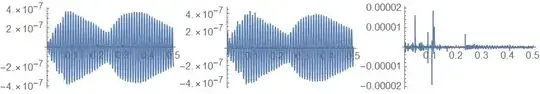
The errors in displacement and velocity are of order 10^-7 which is reasonable but the error in acceleration is of order 10^-5. The errors in acceleration are particularly uneven with significant spikes.

Two equations

The differential equation is now split into two equations, one for displacement and one for velcity.

{d2, v2} = {y, v} /. First@NDSolve[{
       y'[t] == v[t],
       v'[t] + 2 b v[t] + (2 \[Pi] a)^2 y[t] == 0,
       y[0] == y0, v[0] == v0} /. vals, {y, v}, {t, 0, tmax}];
Row[{
  Plot[d2[t] - de, {t, 0, tmax}],
  Plot[(v2[t] - ve)/vmax, {t, 0, tmax}],
  Plot[(v2'[t] - ae)/amax, {t, 0, tmax}]
  }]

The accuracy is worse for the displacement and velocity and no better for the acceleration.

Three equations

Here we have differential equations for the velocity and acceleration. The interaction between these derivatives is expressed as an algebraic equation.

{d3, v3, ac3} = {y, v, ac} /. First@NDSolve[{
       v'[t] == ac[t],
       y'[t] == v[t],
       ac[t] + 2 b v[t] + (2 π a)^2 y[t] == 0,
       y[0] == y0, v[0] == v0} /. vals, {y, v, ac}, {t, 0, tmax}];
Row[{
  Plot[d3[t] - de, {t, 0, tmax}],
  Plot[(v3[t] - ve)/vmax, {t, 0, tmax}],
  Plot[(ac3[t] - ae)/amax, {t, 0, tmax}]
  }]

For this simulation the three results are of order 10^-6 and there are no spikes on any of the simulations. I guess the issues I am seeing are to due to the type of interpolation used. Derivatives of interpolation functions do not work well.

This suggests that the third approach is best if I want about equal errors for displacement, velocity and acceleration. Is this the best approach? Are there other approaches to getting a good second derivative?

If one had a third order, or forth order differential equation (I sometimes do) should one extend this method?

Edit

Following the suggestion using the answer from I M I have investigated setting the interpolation order. The information from Help is not very clear it states

Use InterpolationOrder->All to get interpolation the same order as the method:

Can anyone explain what this means? What are orders of the method?

I have rerun the case with one equation. This gives:

vmax = 600; amax = 400000;
d1a = y /. First@NDSolve[{
       y''[t] + 2 b y'[t] + (2 \[Pi] a)^2 y[t] == 0,
       y[0] == y0, y'[0] == v0} /. vals, y, {t, 0, tmax}, 
     InterpolationOrder -> All];
Row[{Plot[d1a[t] - de, {t, 0, tmax}],
  Plot[(d1a'[t] - ve)/vmax, {t, 0, tmax}],
  Plot[(d1a''[t] - ae)/amax, {t, 0, tmax}]}]

This is now good with similar errors for all derivatives.

Edit 2 Here is another approach suggested by Michael E2 that uses InterpolationOrder-> All, Method->"ImplicitRungeKutta"

vmax = 600; amax = 400000;
d1b = y /. First@NDSolve[{
       y''[t] + 2 b y'[t] + (2 \[Pi] a)^2 y[t] == 0,
       y[0] == y0, y'[0] == v0} /. vals, y, {t, 0, tmax}, 
     InterpolationOrder -> All, Method -> "ImplicitRungeKutta"];
Row[{Plot[d1b[t] - de, {t, 0, tmax}],
  Plot[(d1b'[t] - ve)/vmax, {t, 0, tmax}],
  Plot[(d1b''[t] - ae)/amax, {t, 0, tmax}]}]

This gives an error of 10^-15 which is as much as one can hope for.

A further suggestion by J.M's ttechnical difficulties is to use Interpolation -> All, Method->"StiffnessSwitching"

vmax = 600; amax = 400000;
d1c = y /. First@NDSolve[{
       y''[t] + 2 b y'[t] + (2 \[Pi] a)^2 y[t] == 0,
       y[0] == y0, y'[0] == v0} /. vals, y, {t, 0, tmax}, 
     InterpolationOrder -> All, Method -> "StiffnessSwitching"];
Row[{Plot[d1c[t] - de, {t, 0, tmax}],
  Plot[(d1c'[t] - ve)/vmax, {t, 0, tmax}],
  Plot[(d1c''[t] - ae)/amax, {t, 0, tmax}]}]

This is rather disappointing as there are spikes showing a huge error. However, if you zoom in, ignoring the spikes the error is about 10^-8.

Answer 1

You can increase interpolation order in NDSolve[], not sure, looks like it should be order + 2 or use All:

vmax = 600; amax = 400000;
d1 = y /. First@NDSolve[{
       y''[t] + 2 b y'[t] + (2 \[Pi] a)^2 y[t] == 0,
       y[0] == y0, y'[0] == v0} /. vals, y, {t, 0, tmax},InterpolationOrder -> 4 (*All*)];
Row[{
  Plot[d1[t] - de, {t, 0, tmax}],
  Plot[(d1'[t] - ve)/vmax, {t, 0, tmax}],
  Plot[(d1''[t] - ae)/amax, {t, 0, 0.5}]}]

Edit

Thanks to @xzczd's comment I've remembered, "InterpolationOrder" is related to "DifferenceOrder", not ODE order.

You can use "ImplicitRungeKutta" or "ExplicitRungeKutta" methods, with custom "DifferenceOrder" and "InterpolationOrder" -> All.

For example, this is order 20 adaptive step implicit RK (also symplectic):

Method->{"ImplicitRungeKutta",DifferenceOrder->20,"Coefficients"->"ImplicitRungeKuttaGaussCoefficients","ImplicitSolver"->{"Newton",AccuracyGoal->MachinePrecision,PrecisionGoal->MachinePrecision,"IterationSafetyFactor"->1}}

You can also use fixed step method:

Method->{"TimeIntegration"->{"FixedStep",Method->{"ImplicitRungeKutta",DifferenceOrder->10,"Coefficients"->"ImplicitRungeKuttaGaussCoefficients","ImplicitSolver"->{"Newton",AccuracyGoal->MachinePrecision,PrecisionGoal->MachinePrecision,"IterationSafetyFactor"->1}}}}

For fixed step also set "StartingStepSize", "MaxStepFraction" and "MaxSteps" options.