StreamPlot in Polar Coordinates

Question

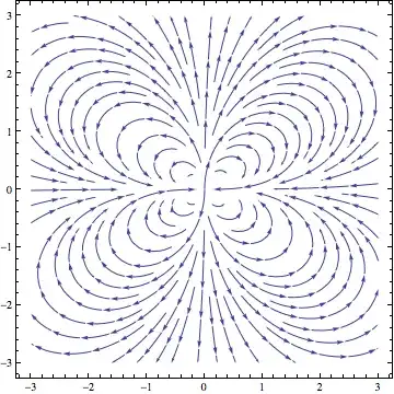
I want to use StreamPlot to map out the field lines of an electric field $\mathbf{E}$ given by $$ \mathbf{E} = \frac{3D}{4r^{4}}(3\cos(\theta)^{2}-1)\mathbf{\hat{r}} +\frac{3D}{4r^{4}}\sin(2\theta)\boldsymbol{\hat{\theta}} $$ I could convert it to Cartesian coordinates, but I have quite a few more fields to plot, so I would rather leave it in polar coordinates. How can I get StreamPlot to accept polar coordinates?

Answer 1

If you have version 9, the TransformedField as mentioned by MichaelE2 is the way to go. In version 8, the analogous thing (which can also still be used in version 9), is this:

Needs["VectorAnalysis`"]
Clear[field, r, θ, ϕ];
m = Transpose[
     Transpose[JacobianMatrix[#, Spherical @@ #]]/
      ScaleFactors[Spherical @@ #]] &@{r, θ, ϕ};
field[r_, θ_, ϕ_] = 
  Simplify[m.{3/(4 r^4) (3 Cos[θ]^2 - 1), 
     3/(4 r^4) Sin[2 θ], 0}];

StreamPlot[
 Delete[
  field @@ CoordinatesFromCartesian[{x, 0, z}, Spherical], 2], 
  {x, -3, 3}, {z, -3, 3}]

It uses the VectorAnalysis package like Spawn's answer, but I didn't see any reason why you would first plot the function in polar coordinates, so I inserted the coordinate transformation directly in the StreamPlot. This works for any field defined as a function (field) of the three spherical coordinates, as shown above. All you need is to replace field by field @@ CoordinatesFromCartesian[{x, y, z}, Spherical]. In the plot here, I just set y=0 to get the field lines in the x-z plane.

Edit

The field in the question was given in spherical coordinates, but I copied it from a comment and assumed it was cartesian components. So to correct that, in the definition of field, I added the transformation to the spherical unit vectors. I did this in the most general way I could think of, so that the field can be changed easily. All that you need is the transformation matrix m. If you desire any other coordinate system, just replace Spherical above.

The definition of field also is kept three-dimensional for generality, so that in the StreamPlot I have to Delete one of the three components. Since I'm plotting the x-z plane, I drop the y component which is zero there.

Answer 2

One way to do it is to write our own wrapper function which does the conversion and feeds it to StreamPlot. Thereby we have the convenience of a selfcontained function without the hassle of having to do the conversion manually every time. We can convert our field

field =  3/(4r^4) (3Cos[\[Theta]]^2-1) OverHat[r]
       + 3/(4r^4) Sin[2\[Theta]] OverHat[\[Theta]]

to cartesian form by preparing a set of conversion rules from polar to cartesian coordinates

tocartesian = {OverHat[r] -> x/r OverHat[x] + y/r OverHat[y],
               OverHat[\[Theta]] -> -(y/Sqrt[x^2+y^2]) OverHat[x]+x/Sqrt[x^2+y^2] OverHat[y],
               r -> Sqrt[x^2+y^2],
               \[Theta] -> ArcTan[x,y] };

and a rule to make this into a list afterwards

cartesianlist = (a_ OverHat[x] + b_ OverHat[y]) -> {a, b};

Then we can let Mathematica repeatedly apply (//.) our tocartesian rule to eliminate all occurences of r and then let FullSimplify help us to eliminate the trigonometric functions. At last we use cartesianlist to switch to list form:

cartesianfield = FullSimplify[field //. tocartesian] /. cartesianlist

For convenient usage we define our own PolarStreamPlot function

PolarStreamPlot[{rfield_,thetafield_}, opts___] := Module[
  {tocartesian,cartesianlist,field,cartesianfield},
  tocartesian={OverHat[r]->x/r OverHat[x]+y/r OverHat[y],
               OverHat[\[Theta]]->-(y/Sqrt[x^2+y^2])OverHat[x]
                                        + x/Sqrt[x^2+y^2] OverHat[y],
               r->Sqrt[x^2+y^2], \[Theta]->ArcTan[x,y]};
  cartesianlist=(a_ OverHat[x] + b_ OverHat[y])->{a,b};
  field = rfield OverHat[r] + thetafield OverHat[\[Theta]];
  cartesianfield = FullSimplify[field//.tocartesian]/.cartesianlist;
  StreamPlot[cartesianfield, opts]
]

and now we can feed it our original $r$-$\theta$ field definition directly

PolarStreamPlot[
  {3/(4r^4) (3Cos[\[Theta]]^2-1),
   3/(4r^4) Sin[2\[Theta]]},
  {x, -3, 3}, {y, -3, 3}
]

Answer 3

Update - A straightforward alternative

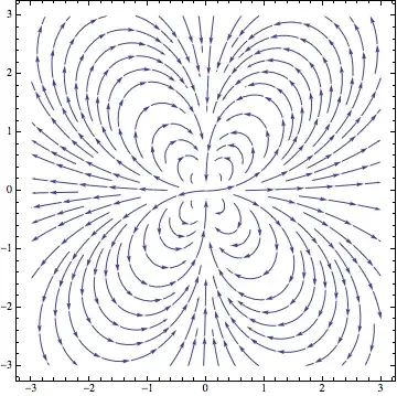
Just to put my comment into code in at least one answer: For V9+,

field = {3/(4 r^4) (3 Cos[θ]^2 - 1), 3/(4 r^4) Sin[2 θ]};
StreamPlot[Evaluate@TransformedField["Polar" -> "Cartesian", 
   field, {r, θ} -> {x, y}], {x, -3, 3}, {y, -3, 3}]
(*  image as above  *)

---

Original approach

Here is an approach I have been taking with my differential equations class. It shows some of the versatility of the Dt operator and we can break the process down into elementary mathematical steps, instead of using TransformedField as a black box, although using Dt to handle the calculus. We can represent $\mathbf{\hat{r}}$ and $\boldsymbol{\hat{\theta}}$ by Dt[r] and r Dt[θ]. Then straight substitutions may be used. In the end we can convert to a vector field by replacing Dt[x], Dt[y] by {1, 0}, {0, 1} respectively.

polarToCartesian = {r -> Sqrt[x^2 + y^2], θ -> ArcTan[x, y]};
differentialTofield = {Dt[x] -> {1, 0}, Dt[y] -> {0, 1}};

field = (3/(4 r^4) (3 Cos[θ]^2 - 1)) Dt[r] + (3/(4 r^4) Sin[2 θ]) r Dt[θ];

cartesianField = 
 field /. polarToCartesian /. differentialTofield // Simplify
(*
  { (3 x ( 2 x^2 - 3 y^2)) / (4 (x^2 + y^2)^(7/2)),
   -(3 y (-4 x^2 +   y^2)) / (4 (x^2 + y^2)^(7/2))}
*)

StreamPlot[
 cartesianField,
 {x, -3, 3}, {y, -3, 3}
 ]

---

Answer 4

Ok the stream plot on the polar space is given by say

With[{D=1},plot=StreamPlot[{3*D/(4r^4)(3Cos[θ]^2-1),3*D/(4r^4) Sin[2θ]},{r,0,1},{θ,0,2*π},
     StreamScale -> {Automatic, Automatic, Automatic, Function[{x, y, vx, vy, n}, x]}]]

Now, IF you want this stream plot embedded on cartesian space you can either transform the vector field to cartesian space as you correctly say or do the following:

Needs["VectorAnalysis`"]
Show[plot/.
Arrow[v:{__?VectorQ}]:>Arrow[(Most[CoordinatesToCartesian[Append[#, 0], Cylindrical]]&/@v)], 
PlotRange -> Automatic]

I suppose your question is if there is a function like PolarPlot for StreamPlot or other plot functions. The short answer is no. You can either change before hand the function or the field or embed the field afterward. Which method is best depends on the specific trasformation involved and if you want to exploit Mathematica's routines in giving you the best presentation of the field.

Answer 5

For those using Mathematica 9, I have created the following function to produce polar plots. It takes all options that can be given to StreamPlot, but also masks any results outside of the provided domain (which is provided in polar coordinates).

SetAttributes[PolarStreamPlot, HoldAll];
PolarStreamPlot[
  fns_, {r_Symbol, rMin_, rMax_}, {t_Symbol, tMin_, tMax_}, opts___] :=
  Module[{Fns, x, y, RF, TMin, TMax, mArcTan, RMax},
  If[rMin >= rMax,
   Throw["Invalid range for r!"]
   ];
  If[tMin >= tMax || tMax - tMin > 2 Pi,
   Throw["Invalid range for \[Theta]!"]
   ];
  TMin = Mod[tMin, 2 Pi, tMin];
  TMax = Mod[tMax, 2 Pi, tMin];
  If[TMax == TMin, TMax += 2 Pi];
  mArcTan[vars__] = Mod[ArcTan[vars], 2 Pi, TMin];
  Fns = TransformedField["Polar" -> "Cartesian", 
     fns, {r, t} -> {x, y}] /. ArcTan -> mArcTan;
  RMax = rMax;
  StreamPlot[Fns, {x, -RMax, RMax}, {y, -RMax, RMax}, 
   RegionFunction -> 
    Function[{x, y}, 
     Evaluate[
      mArcTan[x, y] <= TMax && rMin <= Sqrt[x^2 + y^2] <= rMax]], opts]
  ]

Hope this helps!