Merging two NDSolve solutions

Question

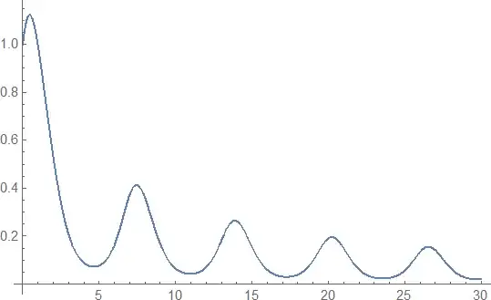
I am trying to merge two NDSolve solutions (solutions of the same problem on a partitioned region). Even though my code does the job, it does it with errors. I was wondering if there are other efficient methods of achieving the same goal.

s1 = NDSolve[{y'[x] == y[x] Cos[x + y[x]], y[0] == 1}, y, {x, 0, 15}];
s2 = 
  NDSolve[
    {y'[x] == y[x] Cos[x + y[x]], y[15] == 0.1546793160063605`}, 
    y, {x, 15, 30}];
ss[x_] := Piecewise[{{s1, x <= 15}, {s2, x >= 15}}];
Plot[Evaluate[y[x] /. ss[x]], {x, 0, 30}, PlotRange -> All]

Possible duplicate: https://mathematica.stackexchange.com/questions/19042/how-to-splice-together-several-instances-of-interpolatingfunction — Michael E2, Dec 18 '20 at 04:30
{{y->InterpolatingFunction[<<5>>]}} x>=15 0 True } is neither a list of replacement rules nor a valid dispatch table, and so cannot be used for replacing.``` — Oluwaseun Sharomi, Dec 18 '20 at 05:43

score 3 · Answer 1 · answered Dec 18 '20 at 07:18

Try NDSolveValue

s1 = NDSolveValue[{y'[x] == y[x] Cos[x + y[x]], y[0] == 1}, y, {x, 0, 15}]
s2 = NDSolveValue[{y'[x] == y[x] Cos[x + y[x]], y[15] == s1[15](*0.1546793160063605`*)},y, {x, 15, 30}]
ss[x_] := Piecewise[{{s1[x], x <= 15}, {s2[x], x > 15}}]
Plot[ss[x], {x, 0, 30}, PlotRange -> All]

Anton Antonov · Answer 2 · 2020-12-19T12:43:35.893

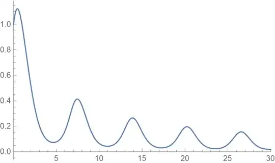
In this particular case instead of using Piecewise we can combine the two solutions by:

Merging the data of the solutions InterpolationFunction objects
Make an InterpolationFunction object with the merged data

Block[{s1 = s1[[1, 1, 2]], s2 = s2[[1, 1, 2]]},
  sss = Interpolation @ Union @ Transpose @
    Map[Flatten, {{s1["Grid"], s2["Grid"]}, 
                  {s1["ValuesOnGrid"], s2["ValuesOnGrid"]}}]
];
Plot[sss[x], {x, 0, 30}, PlotRange -> All, PlotTheme -> "Scientific"]

score 1 · Answer 3 · answered Dec 18 '20 at 08:10

I like to call the solutions of NDSolve like the function you are generating (her y) with the addendum 'sol'. So everybody sees what they are representing.

ysol1 = y /. 
   First@NDSolve[{y'[x] == y[x] Cos[x + y[x]], y[0] == 1}, 
 y, {x, 0, 15}];
ysol2 = y /. 
   First@NDSolve[{y'[x] == y[x] Cos[x + y[x]], 
  y[15] == 0.1546793160063605`}, y, {x, 15, 30}];
ss[x_] = Piecewise[{{ysol1[x], x <= 15}, {ysol2[x], x >= 15}}];
Plot[ss[x], {x, 0, 30}, PlotRange -> All]

cvgmt · Accepted Answer · 2020-12-18T08:09:16.020

You can define ss[x] by use the result of s1 and s2

s1 = NDSolve[{y'[x] == y[x] Cos[x + y[x]], y[0] == 1}, y, {x, 0, 15}]
s2 = NDSolve[{y'[x] == y[x] Cos[x + y[x]], 
   y[15] == 0.1546793160063605`}, y, {x, 15, 30}]
ss[x_] := Piecewise[{{y[x] /. s1, x <= 15}, {y[x] /. s2, x >= 15}}];
Plot[ss[x], {x, 0, 30}, PlotRange -> All]

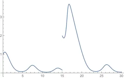
I think you want to change the initial data in the second equations to get another piecewise curves.

s1 = NDSolve[{y'[x] == y[x] Cos[x + y[x]], y[0] == 1}, y, {x, 0, 15}]
s2 = NDSolve[{y'[x] == y[x] Cos[x + y[x]], y[15] == 2}, y, {x, 15, 30}]
ss[x_] := Piecewise[{{y[x] /. s1, x <= 15}, {y[x] /. s2, x >= 15}}];
Plot[ss[x], {x, 0, 30}, PlotRange -> All]

bbgodfrey · Answer 5 · 2020-12-19T04:35:39.340

There are other ways to link the two plots. One is

s1 = NDSolveValue[{y'[x] == y[x] Cos[x + y[x]], y[0] == 1}, y, {x, 0, 15}];
s2 = NDSolveValue[{y'[x] == y[x] Cos[x + y[x]], y[15] == s1[15]}, y, {x, 15, 30}];
Show[Plot[s1[x], {x, 0, 15}, PlotRange -> {{0, 30}, Automatic}],
     Plot[s2[x], {x, 15, 30}]]

Still another is

s12 = Interpolation[{Join[s1["Grid"], s2["Grid"]] // Flatten, 
    Join[s1["ValuesOnGrid"], s2["ValuesOnGrid"]]} // Transpose // Union];

which uses all the y data in s1 and s2. Then, Plot[s12[x], {x, 0, 30}, PlotRange -> All] produces the same curve as above. A similar, although not identical, definition of s12 is

s12 = Interpolation@Join[Table[{x, s1[x]}, {x, 0, 15, .1}], 
    Table[{x, s2[x]}, {x, 15.1, 30, .1}]];

If instead, both the y and y' data in s1 and s2 is desired, then use,

s12 = Interpolation@MapThread[{{#1}, Sequence @@ #2} &, 
    {Join[s1[[3, 1]] // Most, s2[[3, 1]]], 
     Join[Partition[s1[[4, 3]], 2] // Most, Partition[s2[[4, 3]], 2]]}]

which again produces the same result when plotted.

Merging two NDSolve solutions

5 Answers5