Reducing execution time without compromising on accuracy and precision

Question

I have the following NDSolve code, and it is extremely time consuming for me to run it, even when I set both AccuracyGoal and PrecisionGoal to very low numbers such as 3 or 4. Moreover, when I set them at such values, the accuracy and the precision of the result will be compromised greatly, to the extent where my final result is nowhere near what I actually predicted.

The code:

ClearAll["Global`*"]
z[t_] := y[t] - l Cos[φ[t]];
n[t_] := k Abs[z[t]]^(3/2) - c z'[t];
R = 0.0238;
k = 141000000;
c = 20;
g = 9.81;
μk = 0.1804;
i = 6*10^-6;
m = 0.035;
l = R Sqrt[2 (1 + Sin[-(1/2) π - 2*0.3])];
NDSolve[{
  m y''[t] == n[t] - m g,
  φ''[
    t] == (n[t]lSin[φ[t]] + 
      m x''[t]lCos[φ[t]])/i,
x''[t] ==
   If[Abs[(x'[t] + lφ'[t])] < 10^-6 // Evaluate, 
    l (φ''[
          t] Cos[φ[t]] - φ'[t]^2 Sin[φ[
           t]]) // Evaluate, 
    Evaluate@
     If[x'[t] + lφ'[t] > 0, -μkn[t]/m // 
       Evaluate, μkn[t]/m // Evaluate]],
y[0] == l*Cos[0.3], 
  y'[0] == -2.22, φ[0] == 0.3, φ'[0] == -56, 
  x[0] == 0, x'[0] == 0, 
  WhenEvent[z[t] == 0 // Evaluate, "StopIntegration"; Print[y'[t]]; 
   Print[φ'[t]]]}, {y'[t], y[t], x[t], 
  x'[t], φ[t], φ'[t], z[t], 
  n[t], φ''[t]}, {t, 0, 0.2}, 
 Method -> {"EquationSimplification" -> "Residual", 
   "DiscontinuityProcessing" -> False}, AccuracyGoal -> 5, 
 WorkingPrecision -> MachinePrecision, MaxSteps -> 100000000, 
 PrecisionGoal -> 5]

In the nested If statement, I wrote If[Abs[(x'[t] + l*φ'[t])] < 10^-6 // Evaluate instead of If[(x'[t] + l*φ'[t]) ==0 // Evaluate (which is what I actually wanted) where 10^-6 is used as an approximation. It would be good if I can make this number as close to 0 as possible.

In conclusion, is there any method that I can possibly use, to optimise the code and reduce its execution time without compromising on its accuracy and precision? Thank you so much.

Answer 1

Speed tips:

• Explicit is faster than implicit.
• "DiscontinuityProcessing" is your friend.

Other tips:

• WhenEvent is mysterious sometimes, but not here.
• Functions should depend only on their arguments (best practice).
• If 1/10^6 is to be a significant value to NDSolve, AccuracyGoal probably has be somewhat larger than 6.

Irrelevent, gratuitous tips:

• I hate curly phi. :)
• I hope I didn't break anything in refactoring. (Maybe not irrelevant. We'll see.)

Some slight refactoring of the OP's code before converting it to an explicit ODE:

R = 0.0238;
k = 141000000;
c = 20;
g = 9.81;
μk = 0.1804;
i = 6*10^-6;
m = 0.035;
l = R Sqrt[2 (1 + Sin[-(1/2) π - 2*f])];
f = 0.223;
With[{nt = n[z[y[t], phi[t]], D[z[y[t], phi[t]], t]]},
  odeOP = {m y''[t] == nt - m g
    , phi''[t] ==
     1/i (nt l Sin[phi[t]] + m x''[t] l Cos[phi[t]])
    , x''[t] ==
     Simplify`PWToUnitStep@PiecewiseExpand@If[
        Abs[x'[t] + l phi'[t]] < 1/10^6
        , l (phi''[t] Cos[phi[t]] - phi'[t]^2 Sin[phi[t]])
        , -If[x'[t] + l phi'[t] >= 0, 1, -1] (μk nt)/m
        ]}
  ];

Redefine n[], z[]. Differentiate to convert to explicit ODEs. Handle the nondifferentiable functions like Abs and UnitStep. Use odeOP above to fill in missing initial conditions for x''[0] and phi''[0]. NDSolve automatically converts If, Piecewise, UnitStep to discrete events, but I did one of them manually (sgn[t]). I usually don't like Print statements because they can fill a notebook and wrest control from you, if they unexpectedly get out of hand. But I wanted a quick way to check whether an event was detected.

ClearAll[z, n];
z[y_, phi_] := y - l Cos[phi];
n[z_, zp_] := k Abs[z]^(3/2) - c zp;
With[{nt = n[z[y[t], phi[t]], D[z[y[t], phi[t]], t]]},
 odes = {m y''[t] == nt - m g
     , phi'''[t] == D[
       1/i (nt l Sin[phi[t]] + m x''[t] l Cos[phi[t]]) /. 
          {UnitStep -> us, Abs -> abs},
       t]
     , x'''[t] == D[
       Simplify`PWToUnitStep@PiecewiseExpand@If[
           -(1/10^6) < x'[t] + l phi'[t] < 1/10^6
           , l (phi''[t] Cos[phi[t]] - phi'[t]^2 Sin[phi[t]])
           , -sgn[t] (μk nt)/m
           ] /. {UnitStep -> us, Abs -> abs},
       t]
     } /. {us'[_] -> 0, abs' -> (2 UnitStep[#] - 1 &), sgn'[t] -> 0} /.
    {us -> UnitStep, abs -> Abs};
 ics = {y[0] == l Cos[f]
   , y'[0] == -2.22
   , phi[0] == f
   , phi'[0] == -56
   , x[0] == 0
   , x'[0] == 0
   };
 ics = Join[ics, odeOP[[2 ;; 3]] /. t -> 0 /. First@Solve[ics]];
 ics = Join[ics, 
   sgn[0] == Sign[x'[t] + l phi'[t]] /. t -> 0 /. Solve[ics]];
 evts = {WhenEvent[z[y[t], phi[t]] == 0,
    {Print["Stopping at ", t]; "StopIntegration"}]
   , WhenEvent[x'[t] + l phi'[t] > -1/10^6,
    {Print["1" -> {InputForm@t, x'[t] + l phi'[t]}];
     x''[t] -> l (phi''[t] Cos[phi[t]] - phi'[t]^2 Sin[phi[t]])}]
   , WhenEvent[x'[t] + l phi'[t] < -1/10^6,
    {Print["2" -> {InputForm@t, x'[t] + l phi'[t]}];
     x''[t] -> -sgn[t] (μk nt)/m}]
   , WhenEvent[x'[t] + l phi'[t] > 1/10^6,
    {Print["3" -> {InputForm@t, x'[t] + l phi'[t]}];
     x''[t] -> -sgn[t] (μk nt)/m}]
   , WhenEvent[x'[t] + l phi'[t] < 1/10^6,
    {Print["4" -> {InputForm@t, x'[t] + l phi'[t]}];
     x''[t] -> l (phi''[t] Cos[phi[t]] - phi'[t]^2 Sin[phi[t]])}]
   , WhenEvent[x'[t] + l phi'[t] == 0,
    {Print["5" -> {InputForm@t, x'[t] + l phi'[t]}];
     sgn[t] -> -sgn[t]}]};
 ]

Run NDSolve. The monitor is something I use when code takes a long time to run, but it turns out not to be necessary with the "StiffnessSwitching" method. Use the Automatic method, and you can see the stiffness develop just after t = 0.001.

PrintTemporary@Dynamic@{Clock@Infinity, foo};
sol = NDSolve[{odes, ics, evts}
    , {x, y, phi, sgn}
    , {t, 0, 0.2}
    , Method -> "StiffnessSwitching"
    , AccuracyGoal -> 13, (* Note a high AccuracyGoal is needed *)
    WorkingPrecision -> MachinePrecision, 
    PrecisionGoal -> 5, StepMonitor :> (foo = t), 
    DiscreteVariables -> {sgn}, 
    MaxStepFraction -> 1/1000]; // AbsoluteTiming

1->{0.00014391781504231857, -1.*10^-6}  
5->{0.00014391792439061524, 1.19071*10^-14}  
3->{0.00014391803373883832, 1.*10^-6}  

Stopping at 0.000385506

(* {0.085515, Null}  *)

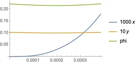
Plot[##, PlotLegends -> {1000, 10, 1} {x, y, phi}] & @@
 {{10000, 10, 1} Through[{x, y, phi}[t]] /. First@sol, 
  Flatten@{t, x@"Domain" /. sol}}

Check events:

Plot @@ {z[y[t], phi[t]] /. First@sol, Flatten@{t, x@"Domain" /. sol}}
Plot @@ {x'[t] + l phi'[t] /. First@sol, Flatten@{t, x@"Domain" /. sol}}
Plot @@ {sgn[t] /. First@sol, Flatten@{t, x@"Domain" /. sol}}

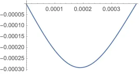
The second one, x'[t] + l phi'[t], controls the If[] statement in the OP (converted to WhenEvents) and sgn[t] and leads to events when its value is ±1/10^6 or 0. The quantity is changing so fast that one wonders if all the events are detected, which was verified by the Print statements in the events. The third plot shows that the sign change in sgn[t] is detected. Here is a visualization of the events. The so-called "signal" is the sign of the event Abs[x'[t] + l phi'[t]] - 1/10^6 == 0 from the If[] statement in the OP's ODE system.

Plot[
 {2/1000000000, 1/2000, 1, 1} {x''[t], x''[t], sgn[t], 
     Sign[Abs[x'[t] + l phi'[t]] - 1/10^6]} /. First@sol // Evaluate,
 {t, 0.00014391775, 0.00014391815},
 PlotPoints -> 200, 
 PlotStyle -> {Thickness@Medium, Thickness@Medium, Directive[Thick], 
   Directive[Dashed, Thick]},
 PlotLegends -> {2./1000000000, 1./2000, 1, 1} {x'', x'', sgn, signal}
 ]