Boundary condition do not satisfied

Question

a = 1;A = 2; Pr = 6.5; M = 1; S = 1; B = 5;
Ode1 = M*(y/2*f''[y] + f'[y]) + f'[y]*f'[y] - f[y]*f''[y] == -A*T'[y]*f''[y] + (a + A)*f'''[y] - A*T[y]*f'''[y];
Ode2 = M*y/2*T'[y] + M*3/2*T[y] + 2*f'[y]*T[y] - f[y]*T'[y] == 1/Pr*(T''[y] + B*T'[y]*T'[y] + B*T[y]*T''[y]);
sol = NDSolve[{Ode1, Ode2, f'[0] == 1, f[0] == S, T[0] == 1, f'[10] == 0, T[10] == 0}, {f, T}, {y}];
Plot[Evaluate[T[y] /. sol], {y, 0, 10}, PlotRange -> All, PlotStyle -> {{Thickness[0.006], Blue}}, AxesOrigin -> {0, 0}, Frame -> True, ImageSize -> Large]

When i run the code for f'[y] it give the correct result, but for T[y] it do not satisfy the boundary conditions

NDSolve gives several error messages "boundary values are not satisfied..." — Ulrich Neumann, Jan 18 '21 at 11:24

score 2 · Accepted Answer · answered Jan 25 '21 at 23:29

We can use Haar wavelets to solve this problem. First we map {y,0,10} on $(0,1)$, then equations turns to

a = 1; A = 2; Pr = 65/10; M = 1; S = 1; B = 5; L = 10;
Ode1 = (-A*T'[y]*f''[y] + (a + A)*f'''[y] - A*T[y]*f'''[y])/L^2 - 
   M*(y/2*f''[y] + f'[y]) - (f'[y]*f'[y] - f[y]*f''[y])/L==0;
Ode2 = 1/Pr*(T''[y] + B*T'[y]*T'[y] + B*T[y]*T''[y])/
     L^2 - (M*y/2*T'[y] + M*3/2*T[y]) - (2*f'[y]*T[y] - f[y]*T'[y])/L==0;

Second step, we define colocation points, wavelets, function and derivatives as follows

J = 4; nn = 2^J; dx = 1/(2*nn); h1[x_] := Piecewise[{{1, 0 <= x <= 1}, {0, True}}]; p1[x_, n_] := (1/n!)*x^n; 
h[x_, k_, m_] := Piecewise[{{1, Inequality[k/m, LessEqual, x, Less, (1 + 2*k)/(2*m)]}, 
    {-1, Inequality[(1 + 2*k)/(2*m), LessEqual, x, Less, (1 + k)/m]}}, 0]
p[x_, k_, m_, n_] := Piecewise[{{0, x < k/m}, {(-(k/m) + x)^n/n!, Inequality[k/m, LessEqual, x, Less, (1 + 2*k)/(2*m)]}, 
    {((-(k/m) + x)^n - 2*(-((1 + 2*k)/(2*m)) + x)^n)/n!, (1 + 2*k)/(2*m) <= x <= (1 + k)/m}, 
    {((-(k/m) + x)^n + (-((1 + k)/m) + x)^n - 2*(-((1 + 2*k)/(2*m)) + x)^n)/n!, x > (1 + k)/m}}, 0]
xl = Table[l*dx, {l, 0, 2*nn}]; xcol = Table[(xl[[l - 1]] + xl[[l]])/2, {l, 2, 2*nn + 1}]; 
f3[x_] := Sum[af[i, j]*h[x, i, 2^j], {j, 0, J, 1}, {i, 0, 2^j - 1, 1}] + a0*h1[x]; 
  f2[x_] := Sum[af[i, j]*p[x, i, 2^j, 1], {j, 0, J, 1}, {i, 0, 2^j - 1, 1}] + a0*p1[x, 1] + f20; 
  f1[x_] := Sum[af[i, j]*p[x, i, 2^j, 2], {j, 0, J, 1}, {i, 0, 2^j - 1, 1}] + a0*p1[x, 2] + f20*x + f10; 
  f0[x_] := Sum[af[i, j]*p[x, i, 2^j, 3], {j, 0, J, 1}, {i, 0, 2^j - 1, 1}] + a0*p1[x, 3] + f20*(x^2/2) + f10*x + f00; 
t2[x_] := Sum[at[i, j]*h[x, i, 2^j], {j, 0, J, 1}, {i, 0, 2^j - 1, 1}] + c0*h1[x]; 
  t1[x_] := Sum[at[i, j]*p[x, i, 2^j, 1], {j, 0, J, 1}, {i, 0, 2^j - 1, 1}] + c0*p1[x, 1] + t10; 
  t0[x_] := Sum[at[i, j]*p[x, i, 2^j, 2], {j, 0, J, 1}, {i, 0, 2^j - 1, 1}] + c0*p1[x, 2] + t10*x + t00;

Third step, we define equations

bc0 = {f1[0] - L, f0[0] - S, t0[0] - 1};
bc1 = {f1[1], 
  t0[1]};(*bc={f'[0]\[Equal]L,f[0]\[Equal]S,T[0]\[Equal]1,f'[1]\
\[Equal]0,T[1]\[Equal]0};*)
var = Flatten[
  Table[{af[i, j], at[i, j]}, {j, 0, J, 1}, {i, 0, 2^j - 1, 1}]];
cons = Join[bc0, bc1];
eqf[y_] := (-A*t1[y]*f2[y] + (a + A)*f3[y] - A*t0[y]*f3[y])/L^2 - 
   M*(y/2*f2[y] + f1[y]) - (f1[y]*f1[y] - f0[y]*f2[y])/L;
eqt[y_] := 
  1/Pr*(t2[y] + B*t1[y]*t1[y] + B*t0[y]*t2[y])/L^2 - (M*y/2*t1[y] + 
     M*3/2*t0[y]) - (2*f1[y]*t0[y] - f0[y]*t1[y])/L;
eq = Join[cons, Flatten[Table[{eqf[x], eqt[x]}, {x, N[xcol]}]]];
varX = Join[{a0, c0, f00, f10, f20, t00, t10}, var];

Finally we compute variables and plot solution

solF = FindRoot[Join[Table[eq[[i]] == 0, {i, Length[eq]}]], 
  Table[{varX[[i]], 1/10}, {i, Length[varX]}]];
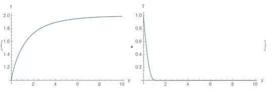
{Plot[f0[x/L] /. solF, {x, 0, 10}, PlotRange -> All, 
  AxesLabel -> {"y", "f"}], 
 Plot[t0[x/L] /. solF, {x, 0, 10}, PlotRange -> All, 
  AxesLabel -> {"y", "T"}]}

thank you so much. Good job. Sir, is this is a specific method how can we function and boundary conditions like this.? — Mathematicain, Jan 27 '21 at 02:40
@Mathematicain You are welcome! This method is more effective to solve BVP, integral equations, fractional differential equations and so on, then that implemented in the current version of NDSolve[]. With this method we can get second numerical solution of your BVP and show why NDSolve can't resolve thermal boundary layer solution like this one. — Alex Trounev, Jan 27 '21 at 09:46
Thank you so much, Dear @Alex. How can we extend this method to the fractional-order derivative? How can then we define f1, f2, ... — Mathematicain, Jan 28 '21 at 10:09
@Mathematicain In a case of fractional derivatives the code is much advanced since differential equation turns to integral equation or integrodifferential equation. I have several examples of such problem solved with Mathematica including this one https://mathematica.stackexchange.com/questions/221609/solver-for-covid-19-epidemic-model-with-the-caputo-fractional-derivatives — Alex Trounev, Jan 28 '21 at 11:56

Boundary condition do not satisfied

1 Answers1