NDSolve big system non linear coupled ODE's Method Residual Stiff System

Question

I'm trying to develop a continuous time unscented Kalman filter for a dynamic system inspired to this article: "On Unscented Kalman Filtering for State Estimation of Continuous-Time Nonlinear Systems" of the author Simo Särkkä. In particular the Square Root one.
My systems has dimension 5 so I have a system of 11 x 5 + 15 non linear coupled first order differential equations.
The code of my notebook is very long and laborious, in the end I simulate a dynamic system and the filter receive the output.
When I try to solve the system with NDSolve it says:

So I do as recommended and it works till it find a singularity that I think is just numerical and not due to the system.
Maybe using Chop to simplify the approximations as I saw in other posts.

This is a short versione of my code:

t0 = 0;
tfin = 4 Pi;
pstl = {xstl, ystl};
R0l[\[Theta]_] = {{Cos[\[Theta]], -Sin[\[Theta]]} , {Sin[\[Theta]], 
    Cos[\[Theta]]}};
pmk1 = {xmk1, ymk1};
pmk2 = {xmk2, ymk2};
numericalvalues = 
  Thread[{l1, l2, xstl, ystl, xmk1, ymk1, xmk2, ymk2} -> {8, 5, 
     3, -2, 32, 16, -15, 2}];
qalist = {x, y, [Theta], xstls, ystls};
qa[t_] = (ToString[#] <> "[t]") & /@ qalist // ToExpression;
qad[t_] = D[qa[t], t];
qadd[t_] = D[qa[t], t];
v[t_] = 2;
[Omega][t_] = 1;
input[t_] = {v[t], [Omega][t]};
g1 = {Cos[#], Sin[#], 0, 0, 0} & @(#[[3]]) &;
g2 = {0, 0, 1, 0, 0};
dyn = (g1@#v[t] + g2[Omega][t]) &;
pstf = ({#1, #2} + R0l[#3 ].{#4, #5}) &;
h1 = (Sqrt[#.#] &[pmk1 - pstf @@ #]) &;
h2 = (Sqrt[#.#] &[pmk2 - pstf @@ # ]) &;
CreateWhiteNoise[[Mu], s, t0_, tfin_, dt_, p_] := 
 Module[{distr, n = Length[[Mu]], listt, nc, listrn},
    listt = Range[t0, tfin, dt];
    nc = Length[listt];
    distr = MultinormalDistribution[[Mu], s];
    listrn = RandomVariate[distr, nc];
    (Interpolation[Thread[Join[{listt, listrn[[All, #]]}]]][p]) & /@ 
   Range@n
  ] (Just create white noise continuous time sample)
cov = {{0.008, 0}, {0, 
   0.008}}; ((0.008//Sqrt) 3 [Equal] 0.268 [m]*)
media = {0, 0};
noise = CreateWhiteNoise[media, cov, t0, tfin + 0.1, 0.04, t ];
h = {h1@#, h2@#} & ;
hn = (h@# + noise) &;
output[t_] = Join[h@qa[t], hn@qa[t]] /. numericalvalues;
eqdyn = qad[t] == dyn@qa[t];
qa0 = Flatten@{-2, 1, Pi/3, pstl} /. numericalvalues;
eqin = qa[0] == qa0;
monitor = {qa[t], input[t], output[t]};
{state, in, out} = 
  NDSolveValue[{eqdyn, eqin}, monitor, {t, t0, tfin}];
ParametricPlot[state[[1 ;; 2]], {t, t0, tfin}]

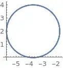
And I get the desired result:

If now I want to use the filter as in the paper:

qlisthat = (ToString@# <> "hat" // ToExpression) & /@ qalist ;
qahat[t_] = (ToString@# <> "[t]" // ToExpression) & /@ qlisthat;
qahatd[t_] = D[qahat[t], t];
nstate = Length@qlisthat;
Covariance Matrix
Pmat = Array[ToExpression[("P" <> ToString[#1] <> ToString[#2])] &, 
   IdentityMatrix[nstate] // Dimensions];
P[t_] = Array[ToExpression[(ToString@Pmat[[#1, #2]] <> "[t]")] &, 
   Dimensions[Pmat]];
Pd[t_] = D[P[t], t];
Initial estimate
P0 = IdentityMatrix[nstate]*{0.005, 0.005, 0.3 Degree, 0.005, 
    0.005 };
stima0 = RandomVariate[MultinormalDistribution[ qa0, P0]];
initstima = qahat[0] == stima0;
initcov = P[0] == P0;
initEKF = {initstima, initcov};
FILTER PARAMETERS AND VARIABLES
k = 1;
[Alpha] = 1;
[Beta] = 0;
nsp = 2 nstate + 1;
[Lambda] = [Alpha]^2 (nstate + k) - nstate;
c = Sqrt[[Alpha]^2 (nstate + k)];
Covariance matrix factorization
decP = SparseArray[{i_, j_} /; i >= j :> 
     ToExpression["a" <> ToString[(10 #1 + #2) &[i, j]]] , 
    Dimensions[Pmat]] // Normal;
Dec[t_] = 
  Array[If[decP[[#1, #2]] == 0, 0 , 
     0, (ToString@decP[[#1, #2]] <> "[t]" ) // ToExpression] &, 
   Dimensions@Pmat];
Decd[t_] = D[Dec[t], t];
Sigma Points
XSP =  SparseArray[{{i_, 
        j_} :> ("xsp"  <> ToString@i <> ToString@j )} , {nsp, 
      nstate}] // Normal // Transpose;
X[t_] = Array[(ToString@XSP[[#1, #2]] <> "[t]" // ToExpression) &, 
   Dimensions@XSP];
Xd[t_] = D[X[t], t];
Sigma points propagation
propX = dyn /@ (X[t][Transpose]) // Transpose // Simplify;
Sigma points output
Ysp = {h1 /@ (X[t][Transpose]), h2 /@ (X[t][Transpose])} /. 
    numericalvalues // Simplify;
z = Transpose@D[hn /@ (X[t][Transpose]), t] /. numericalvalues;
Weights
w0 = [Lambda] / (nstate + [Lambda]);
w = 1 / ( 2 (nstate + [Lambda]));
w0' = w0 + 1 - [Alpha]^2 + [Beta];
wm = Append[{w0}, Table[w, nsp - 1]] // Flatten;
Wm = Table[wm, nsp] // Transpose;
wc = ReplacePart[wm, 1 -> w0'];
Wc = SparseArray[{{1, 1} -> w0', {i_, i_} /; i > 1 -> w}, 
    nsp {1, 1}] // Normal;
W = (IdentityMatrix[nsp] - Wm).Wc.Transpose[
     IdentityMatrix[nsp] - Wm] // Simplify;
FILTER EQUATIONS
[CapitalPhi][mat_] := 
  Module[{i, j}, 
   SparseArray[{{i_, i_} :> mat[[i, i]]/2, {i_, j_} /; i > j :> 
       mat[[i, j]] }, Dimensions[mat]] // Normal];
StackCols[l__?MatrixQ] := MapThread[Join, {l}];
ZeroMatrix[m_, n_] := Normal@SparseArray[{}, {m, n}];
ListForm[mat_] := 
 DeleteCases[(Thread@# & /@ Thread@mat // Flatten ), True]
K = X[t].W. Ysp[Transpose].Inverse[cov];
U = propX.W.X[t][Transpose] + X[t].W.propX[Transpose] - 
   K.cov.K[Transpose];
M = Inverse@Dec[t].U.Transpose[Inverse@Dec[t]];
stimaSRUKBF = X[t].wm;
eqDecP = Decd[t] == Dec[t].[CapitalPhi][M];
eqX = Xd[t] == 
   propX.Wm + K.(z - Ysp.Wm) + 
    c * StackCols[ZeroMatrix[nstate, 1], 
      Dec[t].[CapitalPhi][M], -Dec[t].[CapitalPhi][M]];
eqSRUKBF = {ListForm@eqDecP, eqX};
INITIAL CONDITIONS
A0 = CholeskyDecomposition@P0;
X0 = Transpose[Table[stima0, nsp]] + 
   c * StackCols[ZeroMatrix[nstate, 1], A0, -A0];
initDecp = Dec[0] == A0;
initX = X[0] == X0;
initSRUKBF = {ListForm@initDecp, initX};
INTEGRATION
errstima = qa[t] - stimaSRUKBF;
monitorSRUKBF = {qa[t], stimaSRUKBF, errstima, Xd[t][Transpose]};
(Xd[t] are the derivatives cause singularity)
(With[{opts=SystemOptions[]},Internal`WithLocalSettings[

SetSystemOptions["NDSolveOptions"[Rule]"DefaultSolveTimeConstraint"

[Rule]10.],{stat, statoSRUKBF, errstimaSRUKBF} = NDSolveValue[{eqns, 

eqin, eqSRUKBF, initSRUKBF}, monitorSRUKBF, 
{t,t0,0.04}];,SetSystemOptions[opts]]])
({stat, statoSRUKBF, errstimaSRUKBF} = NDSolveValue[{eqdyn, eqin, 

eqSRUKBF, initSRUKBF}, monitorSRUKBF, 
{t,t0,0.04}];)
{stat, statoSRUKBF, errstimaSRUKBF, der} = 
  NDSolveValue[{eqdyn, eqin, eqSRUKBF, initSRUKBF}, monitorSRUKBF, 
   {t, t0, 0.5}, Method -> {"EquationSimplification" -> "Residual"} ];
(NDSolveValue::ndsz: At t == 0.1982530364128179`, step size is effectively zero; singularity or stiff system suspected.)
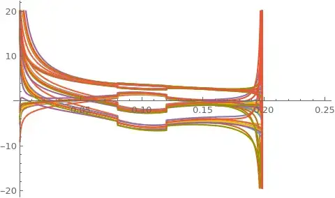
Plot[der, {t, t0, 0.25}]

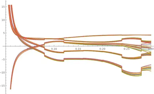
The plot shows the derivatives of the variables that cause singularity. I don't know if is there a way to make the equations in a simpler form that NDSolve can handle, or if is there some trick I can use to manage singularities. The fact is that I think singularity is a numerical matter and not due to the formal system. \

EDIT Replace just these lines of code to make things work:

z = D[hn@qa[t], t] /. numericalvalues // Simplify;
Z = Table[z, nsp] // Transpose;
eqX = Xd[t] == 
  propX.Wm + K.(Z - Ysp.Wm) + 
   c * StackCols[ZeroMatrix[nstate, 1], 
     Dec[t].[CapitalPhi][M], -Dec[t].[CapitalPhi][M]]

And now the system doesn't go on singularity. Before happened because the Dec[t] lost rank during system evolution, but it shouldn't happen, so I've found out the filter's equations weren't right obtaining the following results instead of the previous ones