What is the best way to detect constant or periodic amplitude of the spectrogram?

Question

Suppose I get interpolating function in the solution of the complicated differential system. I plot a solution for various input values that control the outcome of the solution. Some give exponential results and some give sinusoidal results with constant amplitude (periodic) and sinusoidal with increasing amplitude. I am trying to find the solution with constant periodic amplitude. I do that with spectrogram. How do I detect that in spectrogram? In the code, you can see that spectrogram shows constant peaks. I used peak detect for solution of the ode, extrapolated a linear function and calculated the slope of those peaks. But that is time consuming and not a very thorough method. I am looking for another method using spectrogram or other. t1 and t3 shows true and t2 shows false for amplitude detection.

ClearAll;
xrange=40;
ode={y''[x]+a*y'[x]+b*y[x]==0,y'[0]==1,y[0]==0};
solution1=NDSolve[ode/.{a->0.0,b->2},y[x],{x,0,xrange}]
Plot[Evaluate[y[x]/.solution1],{x,0,xrange},PlotRange->All]
solution2=NDSolve[ode/.{a->0.2,b->2},y[x],{x,0,xrange}]
Plot[Evaluate[y[x]/.solution2],{x,0,xrange},PlotRange->All]
Plot[Evaluate[Sin[0.5*x]Cos[6x]],{x,0,xrange},PlotRange->All]
t1=Table[Evaluate[y[x]/.solution1][[1]],{x,0,xrange,1/20}];
Spectrogram[t1]
t2=Table[Evaluate[y[x]/.solution2][[1]],{x,0,xrange,1/20}];
Spectrogram[t2]
t3=Table[Evaluate[Sin[0.5*x]Cos[6x]],{x,0,xrange,1/20}];
Spectrogram[t3]

I.M. · Answer 1 · 2021-04-21T03:03:13.423

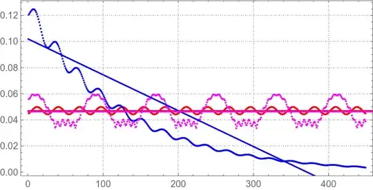
Fitting a slope works fine for your examples. But this approach will fail if sample data contains only a few periods of the slowest component. Some preprocessing might be useful, like removing a mean and using a window function (should improve amplitude estimation accuracy).

Have a look at Prony's decomposition, it can be used to estimated dumping exponents.

Another possibility is to convert your system to a discrete map and study the eigenvalues of its period-1 fixed points.

(* test data *)
ClearAll;
xrange = 40;
range = Subdivide[0, xrange, 512 - 1] ; 
ode = {y''[x]+a*y'[x]+b*y[x]==0,y'[0]==1,y[0]==0};
solution1 = NDSolveValue[ode/.{a->0.0,b->2}, Table[y[x], {x, range}],{x,0,xrange}, Method -> {"FixedStep", Method->Automatic}] ;
solution2 = NDSolveValue[ode/.{a->0.2,b->2}, Table[y[x], {x, range}],{x,0,xrange}, Method -> {"FixedStep", Method->Automatic}] ;
solution3 = Table[Evaluate[Sin[0.5*x]*Cos[6*x]], {x, range}] ;
(* short-time Fourier transform size )
size = 64 ;
( shift step *)
step = 1 ;
(* normalized list of amplitudes (max bin) *)
ClearAll[amplitude] ;
amplitude[data_] := Normalize[Map[Composition[Max, Abs, Fourier], Partition[data, size, step]]] ;
(* fit slope )
fit1 = Fit[amplitude[solution1], {1, x}, x, NormFunction -> Function[Norm[#, Infinity]]]
fit2 = Fit[amplitude[solution2], {1, x}, x, NormFunction -> Function[Norm[#, Infinity]]]
fit3 = Fit[amplitude[solution3], {1, x}, x, NormFunction -> Function[Norm[#, Infinity]]]
( 0.04707773055542490+3.860878264997249^-10 x )
(* 0.10209465082603414-0.000274818352117 x )
( 0.04652035879823726+6.887031938620644^-9 x )
(* plot normalized amplitudes *)
Show[
    ListPlot[
        {amplitude[solution1], amplitude[solution2], amplitude[solution3]},
        PlotStyle -> {Red, Blue, Magenta}, AspectRatio -> 1/2, PlotTheme -> "Detailed", PlotRange -> All, ImageSize -> 400
    ],
    Plot[{fit1, fit2, fit3}, {x, 0, 1000}, PlotStyle->{Red, Blue, Magenta}]
]

(* AIC ratio as a merit parameter *)
ClearAll[score] ;
score[data_] := With[
    {list = amplitude[data]},
    LinearModelFit[list, {1}, x]["AIC"]/LinearModelFit[list, {1, x}, x]["AIC"]
] ;
score[solution1]
score[solution2]
score[solution3]
(* 1.0004652515910932 *)
(* 0.6925895468097228 *)
(* 1.0003369903109047 *)

What is the best way to detect constant or periodic amplitude of the spectrogram?

1 Answers1