Unwrapping a continuous function given by arg

Question

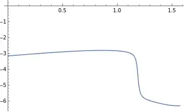
I want to find the Phase difference from a function like $\arg(f(\infty))-\arg(f(0))$ considering the phase jumps in between. This function is continuous but arg might wrap it around, $[-\pi,\pi[$ is there anyway to unwrap a continuous function?

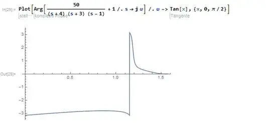
Here is some example code

Plot[Arg[50/((s + 4) (s + 3) (s - 1)) + 1 /. 
    s -> \[ImaginaryJ] \[Omega]] /. \[Omega] -> Tan[x], {x, 
  0, \[Pi]/2}]

I don't necessarily want to plot this function, just do computations with it. But plotting it would be nice too.

Answer 1

Here is a procedure that unwraps your function

f[x_] := Arg[50/((s + 4) (s + 3) (s - 1)) + 1 /. s -> I ω] /. ω -> Tan[x]

We note that Arg is the imaginary part of the logarithm

f[x] /. Arg -> Log
(* Log[1 + 50/((-1 + I Tan[x]) (3 + I Tan[x]) (4 + I Tan[x]))] *)

Of course, the logarithm will still suffer from the same wrapping problem. But we can define an integral which will definitely be continuous.

D[%, x] // FullSimplify
(* (50 I Sec[x]^4 (1 + 4 Cos[2 x] + 6 I Sin[2 x]))/((I + Tan[x]) (-3 I + 
   Tan[x]) (-4 I + Tan[x]) (38 I + 
   Tan[x] (-5 + Tan[x] (-6 I + Tan[x])))) *)

Having differentiated, we can take the imaginary part

Im[%] // ComplexExpand // FullSimplify
(* (100 Cos[
  x]^2 (4397 + 7485 Cos[2 x] + 4426 Cos[4 x] + 1647 Cos[6 x] + 
   285 Cos[8 x]))/((5 + 4 Cos[2 x]) (17 + 
   15 Cos[2 x]) (5297 Cos[2 x] + 5 (682 + 474 Cos[4 x] + 95 Cos[6 x]))) *)

Now we need to integrate. This is conveniently done over the relevant interval by defining and solving a simple differential equation

NDSolveValue[y'[x] == % && y[0] == f[0], y, {x, 0, π/2}];

Giving a result in line (I hope) with what you showed

Plot[%[x], {x, 0, π/2}]

(I think that whether we start at `±π' is down to differences in rounding)

Answer 2

Unfortunately this is not very easy to do. So, I first give the function and then I explain the pieces.

The input consists of: function whose argument is to be searched, start and end of definition domain, number of sampling points.

myArg[fun_, start_, end_, steps_ : 100] := 
  Module[{eps, f, t, s1, s2, xs, d, x, shift, p, t1, t2}, 
   eps = (end - start)/10^6;
   f[x_] := Arg[fun[x]];
   xs = Range[start, end, (end - start)/steps];
   d = f /@ xs // N;
   p = FindPeaks[d][[All, 1]]; p = Select[p, 1 < # < Length[d] &];
   p = Quiet[
       FindMaximum[f[x], {x, #}, Method -> "PrincipalAxis"][[2, 1, 
         2]]] & /@ (xs[[#]] & /@ p);
   {shift, p} = 
    If[Length[#] == 0, {{}, {}}, Transpose[#[[1]]]] &[(Reap[
           Scan[
             (t1 = f[# - eps]; t2 = f[# + eps];
                 If[
                   Abs[t1 - t2] > 6.27, If[
                     t1 < t2, Sow[{-2. Pi, #}], Sow[{2. Pi, #}]]]) &, 
         p]])[[2]]];
   PrependTo[shift, 0];
   shift = Accumulate[shift];
   t = MapIndexed[{f[x] + shift[[Sequence@#2]], x <= #1} &, p];
   t = Map[Flatten, t, 2];
   AppendTo[t, {f[x] + shift[[-1]], True}];
Evaluate[Piecewise[t] /. x -> #] &];

We may test this e.g.:

f[x_] = If[x > 4 Pi, Exp[ I x], Exp[-I x]];
f1[x_] = myArg[f, 0, 20][x];
Plot[{Arg[f[x]], f1[x]}, {x, 0, 20}, PlotRange -> All]

Blue is the original Arg and orange myArg

Now the explanation:

First the definition domain of myArg is coarsely sampled and peaks in the argument are searched. Then the peak locations are determined more accurately and a check is made if the argument changes by 2 Pi. This info is used to calculate a shift that needs to be added do Arg to make myArg continuous. Finally an anonymous function is assembled. Here are the details

For convenience eps and f are defined.

Then a bunch of sampling points: xs and d are calculated. These are used for a coarse for maxima of f:

xs = Range[start, end, (end - start)/steps];
d = f /@ xs // N;
p = FindPeaks[d][[All, 1]]; 
p = Select[p, 1 < # < Length[d] &];

The found coarse maxima are then determined more accurately. We need the method "PrincipalAxis" that does not use derivatives:

p = Quiet[FindMaximum[f[x], {x, #}, Method -> "PrincipalAxis"][[2, 1, 
       2]]] & /@ (xs[[#]] & /@ p);

Then a check is made if the arguments jumps by 2 Pi and if yes the necessary shifts to make myArg continuous are stored:

{shift, p} = Reap[Scan[(t1 = f[# - eps]; t2 = f[# + eps];
        If[Abs[t1 - t2] > 6.27, 
         If[t1 < t2, Sow[{-2. Pi, #}], Sow[{2. Pi, #}]]]) &, p]][[2, 
     1]] // Transpose;
PrependTo[shift, 0];
shift = Accumulate[shift];

With this information the body of a piecewise function is created and the last statement creates the function and makes it an anonymous function:

t = MapIndexed[{f[x] + shift[[Sequence@#2]], x <= #1} &, p];
t = Map[Flatten, t, 2];
AppendTo[t, {f[x] + shift[[-1]], True}];
Evaluate[Piecewise[t] /. x -> #] &
t = MapIndexed[{f[x] + shift[[Sequence@#2]], x <= #1} &, p];
t = Map[Flatten, t, 2];
AppendTo[t, {f[x] + shift[[-1]], True}];
Evaluate[Piecewise[t] /. x -> #] &

Answer 3

As an alternative approach, you could fix up the graph rather than the function. (PlotRange->All ensures that the entire curve is visible)

unwrap[plot_Graphics] := Show[plot /. line_Line :> unwrap[line], PlotRange -> All]
unwrap[line_Line] := Module[{xs, ys},
  xs = First /@ First[line];
  ys = Last /@ First[line];
  Line[Transpose[{xs, unwrap[ys]}]]]
unwrap[ys_List] := Accumulate[Prepend[Mod[Differences[ys], 2 π, -π], First[ys]]]

Try it with the function you specified

f[x_] := Arg[50/((s + 4) (s + 3) (s - 1)) + 1 /. s -> I ω] /. ω -> Tan[x]
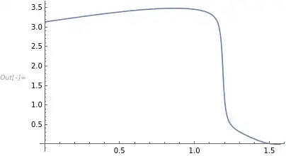
unwrap[Plot[f[x], {x, 0, π/2}, Exclusions -> None]]

I find Exclusions->None is need to give a connected curve (you didn't seem to need it). Since the curve starts from a phase of about -π, whether we get this curve or one 2π larger depends on rounding.