On the numerical roots of transcendent functions

Question

Writing:

{a, b, c, d, e, f, g} = {-2, 2, -2, 2, 0, 6, 5} / 6;
h[t_] := (a + b t + Cos[e + f t])^2 + (c + d t + Sin[e + f t])^2 - g^2
sol1 = NSolve[h[t] == 0, Reals, WorkingPrecision -> 10][[All, 1, 2]]

instantly we get:

{-0.1995415116, 0.6420342510, 3.052979574, 4.390122149}

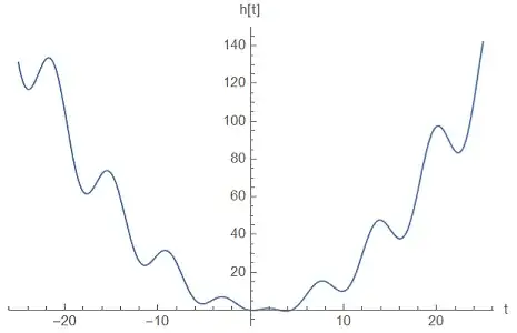
which are all real roots of this function as graphically verifiable:

Plot[h[t], {t, -25, 25}, AxesLabel -> {"t", "h[t]"}]

The best I can do to emulate NSolve[] is to apply the Bolzano's theorem coupled with the Newton-Raphson method:

sol2 = {};
T = 5;
dt = 10^-1;
tol = 10^-10;
ti = -T;
tf = -T + dt;
While[tf < T,
      If[h[ti] h[tf] < tol,
         t0 = (ti + tf) / 2.;
         While[Abs[h[t0] / h'[t0]] > tol,
               t0 = t0 - h[t0] / h'[t0]
              ];
         sol2 = Join[sol2, {t0}]
        ];
      ti = tf;
      tf = tf + dt
     ]
sol1 == sol2

True

but it's evident that all depends heavily on the choice of parameters 0 < dt < T.

The question is therefore how to improve this approach or what other methods I could apply automatically to have the same solutions of NSolve[], as far as possible of course, I understand well that Mathematica algorithms will always be better than my "toys".

---

Addendum

I was very fascinated by the methods suggested in the comments by @Michael E2. While the "graphical methods" are linked to the Plot[] functions implemented internally to Mathematica, the "spectral methods" are potentially exportable in less advanced spreadsheets.

In particular, aware of my limitations and without any pretense, implementing the Chebyshev-proxy rootfinder algorithm in the following way, the idea is to generate the coefficients of a polynomial that in a given interval has the same real roots as the assigned transcendent function, easily computable, for example, with Aberth-Ehrlich method, then adjust with the evergreen Newton-Raphson method:

(*Roots search range and tolerance*)
{tmin, tmax} = {-5, 5};
tol = 10^-10;
n = 10;
While[True,
  (*Calculate Chebyshev's nodes*)
  chebnodes = ConstantArray[0, n + 1];
  For[i = 1, i <= n + 1, i++,            
      ti = Cos[Pi (i - 1) / n] (tmax - tmin) / 2 + (tmax + tmin) / 2.;
      chebnodes[[i]] = h[ti]
     ];

  (*Calculate Chebyshev's coefficients*)
  chebcoeff = ConstantArray[0, n + 1];
  For[i = 1, i <= n + 1, i++,
      sum = 0;
      For[j = 2, j <= n, j++,
          sum = sum + Cos[Pi (i - 1) (j - 1) / n] chebnodes[[j]];
         ];                   
      chebcoeff[[i]] = (chebnodes[[1]] + 2 sum + (-1)^(i-1) chebnodes[[n+1]])/n
     ];
  chebcoeff[[1]] = chebcoeff[[1]] / 2;
  chebcoeff[[n + 1]] = chebcoeff[[n + 1]] / 2;

  (*Calculate error*)
  err = 0;
  For[i = 2 + n/2, i <= n + 1, i++,
      err = err + Abs[chebcoeff[[i]]]
     ];

  (*Check if it's necessary to double the nodes*)
  If[err > tol, n = 2 n, Break[]]
 ];


(Calculate coefficients of resolving polynomial)
polycoeff = ConstantArray[0, n + 1];
For[i = 1, i <= n + 1, i++,
    k = i;
    For[j = 1, j <= (5 + 2 (n - i) - (-1)^(n + i)) / 4, j++,
        If[i == 1,
           l = 1,
           l = 2^i (i + 2 j - 3) (i + j - 3)! / (4 (i - 1)! (j - 1)!)
          ];
        polycoeff[[i]] = polycoeff[[i]] - (-1)^(n + j) l chebcoeff[[k]];
        k = k + 2
       ]
   ];
(Calculate polynomial's roots with Aberth-Ehrlich method)
poly = 0;
For[i = 1, i <= n + 1, i++,
    poly = poly + polycoeff[[i]] t^(i - 1)
   ];
polyroots = {ToRules[NRoots[poly == 0, t, Method -> "Aberth"]]}[[All, 1, 2]];
(Select real roots within the interval)
sol = ConstantArray[0, Length[polyroots]];
nsol = 0;
For[i = 1, i <= Length[polyroots], i++,
    If[-1.001 < Re[polyroots[[i]]] < 1.001 && Abs[Im[polyroots[[i]]]] < 10^-15,
       nsol = nsol + 1;
       sol[[nsol]] = polyroots[[i]] (tmax - tmin) / 2 + (tmax + tmin) / 2
      ]
   ];
(Roots adjustment with Newton-Raphson method)
sol3 = ConstantArray[0, nsol];
For[i = 1, i <= nsol, i++,
    t0 = sol[[i]];
    While[Abs[h[t0] / h'[t0]] > tol,
          t0 = t0 - h[t0] / h'[t0]
         ];
    sol3[[i]] = t0
   ];
sol1 == sol3

True

It's undoubtedly a "toy code", from which, however, I had (and maybe others will have in the future) interesting ideas, most likely new notions compared to the classic "lessons for engineers".

Answer 1

NSolve for a given range of t solves your problem:

 NSolve[{h[t] == 0, -10 < t < 10}, t]
 (*{{t -> -0.199542}, {t -> 0.642034}, {t -> 3.05298}, {t -> 4.39012}}*)