Find FT and r.m.s noise of a signal

Question

I have a signal :

v = 50;
x = 2;
tstart = 0;
tend = 0.45;
num = 256;
tstep = (tend - tstart)/(num - 1) // N;
sig = N[Table[{t, (Exp[-(I*2*Pi*v + Pi*x) (t)] + 
       Random[NormalDistribution[0, .06]] + 
       I Random[NormalDistribution[0, .06]])}, {t, tstart, tend, 
     tstep}]];
ListPlot[Re[sig], PlotRange -> All, Joined -> True]

I need to plot Fourier transform of my signal and also calculate rms noise. How do I do that?

I have an idea that one may calculate it from residuals and measure peak to peak distance but no idea how to implement it.

Look at Fourier to get the spectrum. By noise do you mean unwanted background? — Hugh, Jun 11 '21 at 19:27
@Hugh Ya the root mean square noise (technical term) or the mean unwanted background as you said. — tabi_k, Jun 13 '21 at 06:27
Over a short interval the distinction between noise and signal requires more information. One can assume that your signal is narrow band and the noise wide band. Alternatively you can ask to fit the data to a known functional form and call the part of the signal that does not fit noise. You need to tell us your assumptions. — Hugh, Jun 13 '21 at 06:38
I played around with Prony's method for this data. Interesting. I can tease out something almost plausible if I allow for two frequencies and discard one. The issue is that the data is too sensitive to the noise (at least that's true for my rudimentary code). If I bring that noise from .06 to .002 then I can recover the frequency and damping. It is that latter that appears to be so susceptible to noise. Offhand I do not know why. — Daniel Lichtblau, Jun 14 '21 at 16:29
@DanielLichtblau I have to deal with generally higher noise amplitudes. Is it possible for you to show me what you did with the Prony's method. seems interesting — tabi_k, Jun 14 '21 at 17:01

Hugh · Accepted Answer · 2021-06-15T10:56:37.480

I am not sure exactly what you want but one may proceed as follows. I repeat your start.

v = 50;
x = 2;
tstart = 0;
tend = 0.45;
num = 256;
tstep = (tend - tstart)/(num - 1) // N;
sig = N[Table[{t, (Exp[-(I*2*Pi*v + Pi*x) (t)] + 
       Random[NormalDistribution[0, .06]] + 
       I Random[NormalDistribution[0, .06]])}, {t, tstart, tend, 
     tstep}]];
ListPlot[Re[sig], PlotRange -> All, Joined -> True]

Now I am going to take the Fourier transform. I will assume that you only want the real part of the data you generated.

ft = Fourier[Re[sig[[All, 2]]], FourierParameters -> {-1, -1}];
ListLinePlot[Abs[ft[[1 ;; num/2]]], PlotRange -> All]

In order to look for noise it is probably best to use a log plot

ListLogPlot[Abs[ft[[1 ;; num/2]]], PlotRange -> All, Joined -> True]

This looks to have a background level of noise of about 0.005. I have chosen my FourierParameters so that the total modulus squared in the frequency domain equals the total squaredvalue in the time domain. Thus we have

{Re[sig[[All, 2]]] . Re[sig[[All, 2]]], num ft . Conjugate[ft]}
(* {24.4621, 24.4621 + 0. I} *)

So your background level of 0.005 corresponds to the rms value. The assumption is that your decaying signal in the time domain is narrow band in the frequency domain and thus the background level is revealed.

We can check this by regenerating your data without the noise as follows

v = 50;
x = 2;
tstart = 0;
tend = 0.45;
num = 256;
tstep = (tend - tstart)/(num - 1) // N;
sig = N[Table[{t, (Exp[-(I*2*Pi*v + Pi*x) (t)])}, {t, tstart, tend, 
     tstep}]];
ft1 = Fourier[Re[sig[[All, 2]]], FourierParameters -> {-1, -1}];
ListLogPlot[{Abs[ft[[1 ;; num/2]]], Abs[ft1[[1 ;; num/2]]]}, 
 PlotRange -> All, Joined -> True]

The assumption that the signal has dropped below the noise in the frequency domain is just about true.

If you wish to use a complex signal in the time domain you can repeat doing that. Why are you complex in the time domain? It would be interesting to know that.

Hope that helps.

Edit

The OP has complex data in the time domain so we have to take this into account in Fourier.

Starting again we have

v = 50;
x = 2;
tstart = 0;
tend = 0.45;
num = 256;
tstep = (tend - tstart)/(num - 1) // N;
sig = N[Table[{t, (Exp[-(I*2*Pi*v + Pi*x) (t)] + 
       Random[NormalDistribution[0, .06]] + 
       I Random[NormalDistribution[0, .06]])}, {t, tstart, tend, 
     tstep}]];
ListPlot[Re[sig], PlotRange -> All, Joined -> True]
ListPlot[{#[[1]], Im[#[[2]]]} & /@ sig, PlotRange -> All, 
 Joined -> True]

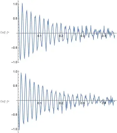
Where both real and imaginary parts are plotted.

Next we take the Fourier transform. It is notable that the OP uses the convention of E^(-I ω t) in the time domain thus indicating that in the FourierParameters the appropriate convention is {-1,1}. If the convention of {-1,-1} is used, common in signal processing, the peak in the spectrum occurs at negative frequencies. Thus

ft = Fourier[sig[[All, 2]], FourierParameters -> {-1, 1}];
{sig[[All, 2]] . Conjugate[sig[[All, 2]]], ft . Conjugate[ft] num}
(* {47.9484 + 0. I, 47.9484 + 0. I} *)

Here I have again checked that the total square in the time domain equals the total square in the frequency domain. Plotting we have

ListLogPlot[{Abs[ft]}, PlotRange -> All, Joined -> True]

So once again we can see that the noise background is about 0.005. Finally we check that the signal with no noise is below the noise floor.

sig1 = N[Table[{t, Exp[-(I*2*Pi*v + Pi*x) (t)]}, {t, tstart, tend, 
     tstep}]];
ft1 = Fourier[sig1[[All, 2]], FourierParameters -> {-1, 1}];
ListLogPlot[{Abs[ft], Abs[ft1]}, PlotRange -> All, Joined -> True]

The OP wants to consider fitting a Lorentzian. There are plenty of other posts that do that.

I work on signals in Magnetic Resonance Spectroscopy and they are complex in time domain. — tabi_k, Jun 14 '21 at 08:29
The Fourier algorithm takes complex data in the time domain so you should be able to use that here. Have I answered your question? If your data can be collected over a longer time interval then the signal would decay into the background noise and the rms noise value would be clearer. Alternatively, can you collect data when there is no signal so that the noise can be identified? — Hugh, Jun 14 '21 at 08:53
I could not get it to work for complex domain but real part seems to be working great. Alternatively I was just trying to fit the data to a Lorentzian and getting the residuals. Yes I can collect data when the signal has decayed completely. But it's not feasible to go that far when doing experiments. — tabi_k, Jun 14 '21 at 16:58

score 2 · Answer 2 · answered Jun 15 '21 at 19:31

Here is an approach to analyzing the signal using Prony's method. This is applicable to data from evenly spaced measurements, when the signal is a sum of complex exponentials. The code is taken from an MSE thread; substantially similar is also in a Wolfram Community thread.

We repeat the code used to obtain signal data.

v = 50;
x = 2;
tstart = 0;
tend = 0.45;
num = 256;
tstep = (tend - tstart)/(num - 1) // N;
noise = .06;
sig = N[Table[{t, (Exp[-(I*2*Pi*v + Pi*x) (t)] + 
       Random[NormalDistribution[0, noise]] + 
       I Random[NormalDistribution[0, noise]])}, {t, tstart, tend, 
     tstep}]];
ListPlot[Re[sig], PlotRange -> All, Joined -> True]

The tricky part is in deciding where to cut off the singular values in the Prony matrix. I opted to allow a bit more than an order of magnitude since that gave a viable result (trial and error).

data = Re[sig][[All, 2]];
len = Length[data];
mat = Most[Partition[data, Floor[len/2], 1]];
tol = 10^(-1.2);
keep = Length[SingularValueList[mat, Tolerance -> tol]]
mat2 = Most[Partition[data, keep, 1]];
rhs = Drop[data, keep];
soln = PseudoInverse[mat2] . rhs;
roots = xx /. NSolve[xx^keep - soln . xx^Range[0, keep - 1] == 0, xx]
(* Out[670]= 8
Out[674]= {-0.646877, -0.592545, -0.387961 - 0.67201 I, -0.387961 + 
  0.67201 I, 0.235216 - 0.698548 I, 0.235216 + 0.698548 I, 
 0.839098 - 0.519868 I, 0.839098 + 0.519868 I} *)

The frequencies of interest are the logarithms of the above roots.

freqs = Log[roots]

(* Out[675]= {-0.435599 + 3.14159 I, -0.523328 + 3.14159 I, -0.253657 - 2.09437 I, -0.253657 + 2.09437 I, -0.30505 - 1.246 I, -0.30505 + 1.246 I, -0.012993 - 0.554674 I, -0.012993 + 0.554674 I} *)

I do not know what to make of those 3.14159 imaginary factors; they do not actually correspond to the frequency terms of interest.

We now obtain amplitudes and construct the sum of complex exponentials signal for the amplitudes and frequencies.

obstime = .45;
timescale = obstime/255;
newmat = Map[roots^# &, Range[0, obstime, timescale]/timescale];
coeffs = Chop[PseudoInverse[newmat] . data]
newf = Chop[coeffs . Exp[freqs*t/timescale]]
(* Out[681]= {1.93284, -2.1813, 0.0349408 - 0.0837537 I, 
 0.0349408 + 0.0837537 I, 0.0701918 - 0.00133477 I, 
 0.0701918 + 0.00133477 I, 0.531129 + 0.0164742 I, 
 0.531129 - 0.0164742 I}
Out[682]= -2.1813 E^((-296.553 + 1780.24 I) t) + 
 1.93284 E^((-246.84 + 1780.24 I) t) + (0.0701918 - 
    0.00133477 I) E^((-172.862 - 706.066 I) t) + (0.0701918 + 
    0.00133477 I) E^((-172.862 + 706.066 I) t) + (0.0349408 - 
    0.0837537 I) E^((-143.739 - 1186.81 I) t) + (0.0349408 + 
    0.0837537 I) E^((-143.739 + 1186.81 I) t) + (0.531129 + 
    0.0164742 I) E^((-7.36267 - 314.316 I) t) + (0.531129 - 
    0.0164742 I) E^((-7.36267 + 314.316 I) t) *)

Several terms are going to die out quite quickly. The last two are the ones of interest.

ListPlot[Table[newf, {t, Range[0, obstime, timescale]}], 
 PlotRange -> All, Joined -> True]

It bears a passing resemblance to the original data.

I rather suspect there are more numerically stable methods one can use. And possibly there are guidelines for how to select that tolerance.

I.M. · Answer 3 · 2021-06-15T20:05:42.843

I rather suspect there are more numerically stable methods one can use. And possibly there are guidelines for how to select that tolerance.

A possible solution is to use optimal SVD truncation for Prony/Hankel matrix. Matan Gavish, David L. Donoho, The Optimal Hard Threshold for Singular Values is 4/sqrt(3)

With SeedRandom[1] approximate (see also a more accurate estimation in the linked ref) rank estimation for unknown noise is two as expected and noise sigma estimation is also close:

ClearAll[optimal$svd$truncation] ;
optimal$svd$truncation[MATRIX_?MatrixQ,SIGMA_Real] := Block[
{NR, NC, LIST, BETA, LAMBDA, TAU},
{NR, NC} = Dimensions[MATRIX] ;
LIST = SingularValueList[MATRIX, Min[{NR, NC}]] ;
BETA = N[Apply[Divide, {NR, NC}]] ;
LAMBDA = Sqrt[2*(BETA + 1) + 8*BETA/(BETA + 1 + Sqrt[BETA^2 + 14*BETA + 1])] ;
TAU = LAMBDA*Sqrt[N[NC]]*SIGMA ;
{Length[DeleteCases[Ramp[Subtract[LIST, TAU]], N[0]]], TAU, SIGMA}
] ;
optimal$svd$truncation[MATRIX_?MatrixQ] := Block[
{NR, NC, LIST, MEDIAN, BETA, LAMBDA, OMEGA, TAU},
{NR, NC} = Dimensions[MATRIX] ;
LIST = SingularValueList[MATRIX, Min[{NR, NC}]] ;
MEDIAN = Median[LIST] ;
BETA = N[Apply[Divide, {NR, NC}]] ;
LAMBDA = Sqrt[2*(BETA + 1) + 8*BETA/(BETA + 1 + Sqrt[BETA^2 + 14*BETA + 1])] ;
OMEGA = 0.56*BETA^3 - 0.95*BETA^2 + 1.82*BETA + 1.43 ;
TAU = OMEGA*MEDIAN ;
{Length[DeleteCases[Ramp[Subtract[LIST, TAU]], N[0]]], TAU, TAU/LAMBDA/Sqrt[N[NC]]}
] ;
optimal$svd$truncation[mat, 0.06] 
optimal$svd$truncation[mat] 
(* {2,1.56767,0.06} *)
(* {2,1.56091,0.0597412} *)

Find FT and r.m.s noise of a signal

3 Answers3