Nonlinear frequency response

Question

I am trying to reproduce the result of this paper, namely Figure 10 which depicts the solution of equation 64 given as,

qmax is the steady state solution of the oscillatory equation given. I tried to reproduce the result using the code below:

data = {Vac -> 0.01 Cos[\[CapitalOmega] t], Vdc -> 100, c -> 0};
 eq = q''[t] + c*q'[t] + 864.82*q[t] + 21.78 q[t]^2 + 142.58 q[t]^3     == 
  45.31 ((2 Vac)/Vdc + Vac^2/Vdc^2) + (1 + (2 Vac)/Vdc + Vac^2/
  Vdc^2)*(123.51 q[t] + 74.09 q[t]^2 + 1424.72 q[t]^3 - 
  122.45 q[t]^4);
sol = ParametricNDSolve[{eq /. data, q[0] == 0, q'[0] == 0}, 
 q, {t, .1, 100}, {\[CapitalOmega]}];
lst={#, Max[q[#][Range[80, 100, .1]] /. sol]} & /@ Range[20, 30, .1];
ListPlot[lst];

As you can see the figure is different. I appreciate if you can help in getting the same figure (figure 10), shown below

Regards,

score 4 · Accepted Answer · answered Jul 17 '21 at 15:14

I have looked into the paper and your code, and I think there are two main issues.

I couldn't have deduced how you obtained the value $V_{dc}=100$, and I also think this is why your results are off. However, neither couldn't I have found the correct value in the paper ($\alpha_2 V^2 = 45, V = V_{ac} + V_{dc}, V_{ac}=0.01$ – this still leaves unknown $\alpha$ and $V_{dc}$).
Your timerange when solving the DE might be too short for some parameter values (very small $c$).

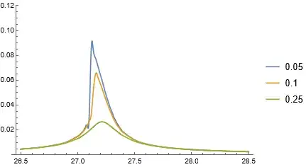
I have tried by some trial-and-error to deduce that $V_{dc} \approx 5$ gives approximately the same results. Be careful, they used two approximation methods (Chebyshev and Taylor) which have slightly different positions of the peak, $\Omega_{\text{Ch.}} \approx 27.1$ and $\Omega_{\text{Tay.}} \approx 27.4$. However, you are solving the DE without approximations and the peak occurs somewhere in between at $\Omega \approx 27.2$.

data = {Vac -> 0.01 Cos[\[CapitalOmega] t], Vdc -> 5};
eq = q''[t] + c*q'[t] + 864.82*q[t] + 21.78 q[t]^2 + 142.58 q[t]^3 == 
   45.31 ((2 Vac)/Vdc + Vac^2/Vdc^2) + (1 + (2 Vac)/Vdc + 
       Vac^2/Vdc^2)*(123.51 q[t] + 74.09 q[t]^2 + 1424.72 q[t]^3 - 
       122.45 q[t]^4);
sol = ParametricNDSolve[{eq /. data, q[0] == 0, q'[0] == 0}, 
   q, {t, .1, 200}, {\[CapitalOmega], c}];
cs = {0.05, 0.1, 0.25};
[CapitalOmega]s = Sort[Union[Range[26.5, 28.5, .1], Range[27, 27.4, .02]]];
lst = Table[{[Omega], First@NMaximize[{q[[Omega], c][t] /. sol, 190 < t < 200}, t]}, 
   {[Omega], [CapitalOmega]s}, {c, cs}];
lst2 = Partition[Transpose@lst, Dimensions[cs]];
ListPlot[First@lst2, PlotRange -> {0, 0.12}, Joined -> True, 
   InterpolationOrder -> 2, PlotLegends -> cs]

I hope you find any of these comments valuable. Note, however, that there might be some more efficient (faster) ways of calculating the maxima; I haven't looked into that.

Many thanks bro. You saved me a lot of time and efforts. I appreciate your help. Many thanks again. — qahtah, Jul 18 '21 at 07:16

Nonlinear frequency response

1 Answers1