My code produces the iconic figure showing the error threshold of the quasispecies model.
Clear["Global`*"]
L = 10
n = L+1
f = ConstantArray[1, n]
f[[1]] *= 10
f
tMax = 10^4
MatrixForm[
q =
Table[
    Sum[
           u ^   (i+j-2k)
        (1-u)^(L-(i+j-2k))
        Binomial[L-i,j-k]*
        Binomial[  i,  k],
        {k,Max[0,i+j-L],Min[i,j]}],
    {i,0,L},{j,0,L}]
]
DiffEqn =
Table[
      Dt[x[i][t], t] == Sum[x[j][t]f[[j]]q[[j,i]], {j,n}] - Sum[x[i][t]f[[i]], {i,n}]x[i][t],
      {i,n}
      ]
solution =
ParametricNDSolve[
    {DiffEqn, Table[x[i][0] == 1/n, {i,n}]},
    Table[x[i], {i,n}],
    {t,0,tMax},
    {u}]
figure =
Plot[Evaluate[Table[x[i][u][tMax], {i,n}]/.solution],
     {u,0,1},
     PlotRange->{{0,1},{0,1}},
     PlotLegends->Placed[Range[n]-1,Below]]
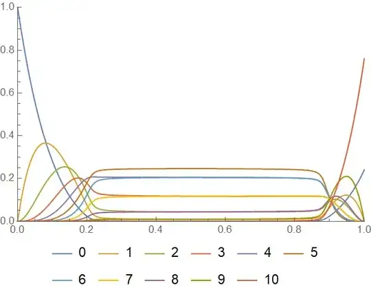
Beautiful.
Now, I would like to add another dimension to the figure by plotting the curves of the different error classes separately along an additional axis.
There are several questions and answers on this site about this, e.g. this Q&A and the questions linked therein. So my question might well be a duplicate.
But I've tried and failed miserably to produce the desired figure based on the other Q&As.
figure2 =
ParametricPlot3D[Evaluate[Table[i-1,u,x[i][u][tMax], {i,n}]/.solution],
                 {u,0,1}]
I don't know where I was mistaken. But I'm not sure I understand how I should use the ParametricFunction objects (produced by ParametricNDSolve) with ParametricPlot3D.
