White noise $\eta(t)$

Question

How to make a random function $\eta(t)$ to insert in a differential equation for NDSolve?

Edit: example: to solve equations like $\frac{dx}{dt}=\eta(t)$

The numerical methods used by NDSolve won't work correctly if you introduce noise. — Szabolcs, May 14 '13 at 19:23
But do take a look here: http://reference.wolfram.com/mathematica/guide/StochasticDifferentialEquationProcesses.html — Szabolcs, May 14 '13 at 19:24
@richard Please still consider adding a minimal example so that someone can perhaps provide an answer using the new stochastic process functions in version 9 (or you can answer your own question as well). That way, it will also be of use to future visitors who have the same problem (I had forgotten as well and was reminded of the new functionality by Szabolcs's link) — rm -rf, May 14 '13 at 19:38
As you've seen, you should have mentioned you're dealing with SDEs at the outset. NDSolve[] indeed does not have SDE-solving capability, but the new functions in 9 will be useful. — J. M.'s missing motivation, May 15 '13 at 04:15
@J.M., thanks, I tried to find a function at least has a quasi-random behavior but i couldn't. But you are saying that even i could find such function, NDSolve won't work? — richard, May 15 '13 at 04:22
Well, it certainly wasn't intended to be used for SDEs. It was, for instance, only relatively recently that NDSolve[] started supporting DAEs and DDEs; maybe a future version might add SDE support, but not now. Thus, you might need to roll your own solution. If you can't or won't use version 9, you may have to implement the Itō process on your own. — J. M.'s missing motivation, May 15 '13 at 04:30

score 10 · Answer 1 · edited Aug 16 '13 at 12:44

10

I think what he means is the following (I could be wrong though). In Mathematica white noise is represented by WienerProcess "also known as Brownian motion, a continuous-time random walk, or integrated white Gaussian noise." ~ Documentation. So adopting (actually simplifying) this example we get the following:

\[ScriptCapitalP] = 
 ItoProcess[\[DifferentialD]x[t] == σ \[DifferentialD]w[t], 
  x[t], {x, x0}, t, w \[Distributed] WienerProcess[]]

 ItoProcess[{{0}, {{σ}}, x[t]}, {{x}, {x0}}, {t, 0}]

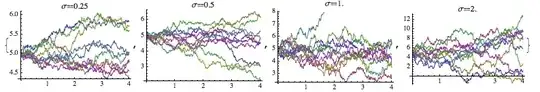
Simulate the process for different values of the variance parameter:

Table[ListLinePlot[
  RandomFunction[\[ScriptCapitalP] /. {x0 -> 5}, {0, 4, 0.01}, 10], 
  PlotLabel -> 
   Row[{"σ", "\[Equal]", N@σ}]], {σ, {1/4, 1/2, 
   1, 2}}]

enter image description here

You can find many characteristics now - see details on the page a linked above, but here is a taste - find the probability density function of the value of the process:

PDF[\[ScriptCapitalP][t], x]

 E^(-((x - x0)^2/(2 t σ^2)))/(Sqrt[2 π] Sqrt[t σ^2])

edited Aug 16 '13 at 12:44

M6299

1,471
1
13
20

answered May 14 '13 at 20:04

Vitaliy Kaurov

73,078
9
204
355

1

Nice, I think this is exactly what the OP was after. Perhaps you could also give this question a shot... – rm -rf May 14 '13 at 20:54
I don't have version 9 – richard May 14 '13 at 21:03
@rm-rf thanks, i will take a look when I get time. That looks like an interesting equation. – Vitaliy Kaurov May 14 '13 at 21:30
@richard maybe you could try a free trial version for now - just to see how it works. – Vitaliy Kaurov May 14 '13 at 21:30
+1 for solving the OP's problem partially, though white noise is not necessarily Gaussian. – Silvia May 15 '13 at 12:07

White noise $\eta(t)$

1 Answers1