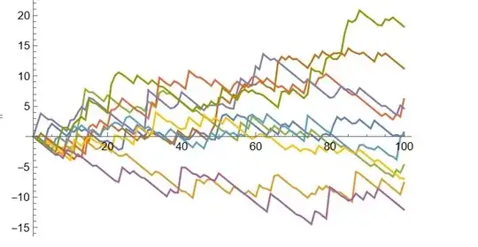
Let us consider the following martingale "compensated compound Poisson process" $M_t=\sum_{k=1}^{N_t} Z_k-\lambda t E(Z)$ where $N_t$ is a Poisson process with intensity $\lambda$, $Z_k$ is iid random variable and indepent with $N_t$.
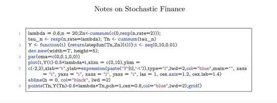
If we consider a special case on "Stochastic Calculus for Jump Processes(https://personal.ntu.edu.sg/nprivault/MA5182/stochastic-calculus-jump-processes.pdf)" P703. We have the following figure  The author get it from software R. You can see the original code from the following picture
  . My problem is that how can I get the similar simulation from Mathematica?
Asked
Active
Viewed 221 times
0
Ailiy Evan
- 103
- 3
-
1Please add the Mathematica code you have tried and the problems you have encountered. – bbgodfrey Aug 02 '21 at 12:52
-
SeedRandom[1]; With[{[Lambda] = 0.6, [Mu] = 0.5, x0 = 1}, proc = ItoProcess[m'[t] = y'[t] - [Lambda] *[Mu], m[t], {m[0], x0}, y [Distributed] CompoundPoissonProcess[ 0.5, ExponentialDistribution[1]]]; rp = RandomFunction[proc, {0., 5., 0.01}]] ListLinePlot[rp] – Ailiy Evan Aug 02 '21 at 16:28
-
Here is the Mathematica code I have tried. But It doe not work. – Ailiy Evan Aug 02 '21 at 16:29
-
Maybe I should not use the ItoProcess. But I have no idea to simulate it. – Ailiy Evan Aug 02 '21 at 17:26
1 Answers
1
TransformedProcess may be helpful.
For example:
p = CompoundPoissonProcess[.5, ExponentialDistribution[1]];
tr = TransformedProcess[x[t] - Mean[p[t]], {x \[Distributed] p}, t];
rf = RandomFunction[tr, {0, 100}, 10];
ListPlot[rf, Joined -> True]
ubpdqn
- 60,617
- 3
- 59
- 148
