Branches of a curve defined implicitly

Question

I have the variable functiontoplot, defined using the following piece of code:

f1 = d*v + u^2*v - u;
f2 = b - d*v - u^2*v;
eq = Solve[{f1 == 0, f2 == 0}, {u, v}][[1]];
jacobianmat = D[{f1, f2}, {{u, v}}];
diffmatrix = DiagonalMatrix[{D1, D2}];
det = FullSimplify[Det[jacobianmat - \[Mu]*diffmatrix]];
der = FullSimplify[D[det, \[Mu]]];
ksquared = Simplify[Solve[der == 0, \[Mu]][[1]]];
D1 = delta^2;
D2 = 1;
delta = 0.045;
functiontoplot = det /. ksquared /. eq;

I want to plot the curve defined by the equation functiontoplot==0. If I use the following line of code:

ContourPlot[functiontoplot == 0, {b, 0, 4}, {d, 0, 6}]

I get the following output:

However, I would like to be able to find and plot these two branches using the function TrackRootPAL explained in the first answer here:

Is there any predictor-corrector method in Mathematica for solving nonlinear system of algebraic equations?

Next, for instance, if I take the initial condition $(b,d)=(0.5,1)$ using the following piece of code:

tr = TrackRootPAL[{functiontoplot}, {d}, {b, 0, 4}, 0.5, {1}];
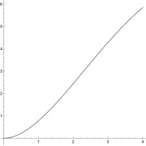
Plot[Evaluate[d[b] /. tr], {b, 0, 4}, AspectRatio -> 1]

then I get the following output:

However I have not been able to find the other branch. In particular, when $(b,d)=(1.87158,5.93002)$, you have that functiontoplot==-0.0000111135. However, if I try to use the following piece of code:

tr = TrackRootPAL[{functiontoplot}, {d}, {b, 0, 4}, 1.87158, {5.93002}];
Plot[Evaluate[d[b] /. tr], {b, 0, 4}]

I get the following Warning:

which produces an empty plot output. Is there a way to solve this problem and be able to find the two branches of the curve in order to use the Pseudo-Arclength Continuation method to plot my curve? I am trying to do this because I want to plot the curve defined implicitly in a quicker way in some cases where functiontoplot could be defined in a messier way.

Answer 1

You can try parametrizing your variables by the arc length. Parametrize your function:

func = functiontoplot /. {b -> b[t], d -> d[t]}

b[t]^2 + d[t] + 123.457 (1 + 0.002025 b[t]^2 + 0.002025 d[t] - (2 b[t]^2)/( b[t]^2 + d[t]))^2 - 246.914 (1 + 0.002025 b[t]^2 + 0.002025 d[t] - (2 b[t]^2)/( b[t]^2 + d[t])) (1 - (2 b[t]^2)/(b[t]^2 + d[t]) + 0.002025 (b[t]^2 + d[t]))

Then, differentiate wrt t to obtain an ODE:

eqn = D[func, t] == 0;

To use NDSolve we need an initial condition:

dvalues = d /. Quiet @ Solve[functiontoplot == 0 /. b->.5, d]

{0.220505, 0.284601, 461.616, 524.534}

Finally, include an arc length constraint and use NDSolve:

sol = NDSolve[
    {
    eqn,
    b'[t]^2 + d'[t]^2 == 1,
    b[0] == .5,
    d[0] == dvalues[[2]]
    },
    {b, d},
    {t, -15, 15}
];

Visualization:

ParametricPlot[{b[t], d[t]} /. sol, {t, -15, 15}, AspectRatio->1]