Aren't roots of polynomial equations smooth functions of their parameters?

Question

I am trying to find the solution of cubic equation as a function of $kz$

-1.05976 + λ (-4.3872 + (-3.9 - 
       1. λ) λ) + (1.10144 + 0.624 λ) Cos[
   1.31 kz] + 0.035152 Cos[2.62 kz]==0

{e1[kz_], e2[kz_], 
  e3[kz_]} = λ /. 
   NSolve[-1.05976 + λ (-4.3872 + (-3.9 - 
       1. λ) λ) + (1.10144 + 0.624 λ) Cos[
   1.31 kz] + 0.035152 Cos[2.62 kz]==0, λ] // FullSimplify

If I plot e1[kz] as function of kz,

Plot[e1[z], {z, 0, π/1.31}]

I get a function that is not smooth. However, if I plot another solution alongside then it seems two solution got mixed up.

Plot[{e1[z], e3[z]}, {z, 0, π/1.31}]

Does anyone know why is this the case? Also, can you fix this?

It is not a bug, it is a feature: blue line is the lower root, orange live is the next one. If you do not like this numerical order, it is possible to resort according to your preferences, which ones? — yarchik, Sep 06 '21 at 22:04
@yarchik I get what you are saying and make sense. But what if I want a solution that is smooth regardless of its value being higher or lower. Is this possible? — sslucifer, Sep 06 '21 at 22:31
The issue we encounter here is well known on the basis of Root objects, which appear behind the scene of NSolve, see e.g. find where 3 inequalities are simultaneously greater than zero but we could find many more posts here regarding this issue. For this reason I recommend changing the title of the question since this might lead to confusion, a better example : "Aren't roots of polynomial equations smooth functions of their parameters?" — Artes, Sep 07 '21 at 23:13

score 6 · Answer 1 · edited Sep 08 '21 at 00:38

With a tip of the hat to @MichaelE2 (from whom I learned this trick), we can differentiate the implicit relation between $\lambda$ and $k_z$ and then solve it as an ODE:

neweq = eq /. λ -> λ[kz];
startkz = π/6;
startval = λ[startkz] /. Solve[neweq /. kz -> startkz, λ[startkz]]
soln = NDSolve[{D[neweq, kz], λ[startkz] == startval}, λ, {kz, 0, π/1.31}, Method -> "StiffnessSwitching"]
Plot[Evaluate[Table[Indexed[λ[kz] /. First[soln], i], {i, 1, 3}]], {kz, 0, Pi/1.31}]

This method may not be entirely robust, but it does seem to work in this case. Notes:

The initial values for the ODE are specified at startkz = Pi/6 in order to ensure that all three roots are distinct at that point and therefore that Mathematica produces three different solutions.
The StiffnessSwitching option is necessary to integrate past the points where the roots cross.
The use of Table and Indexed is required because Mathematica is returning a vector-valued InterpolatingFunction, and some chicanery is needed to get Plot to plot the three components with distinct colors (among other things you might want to do with the result.)

Bob Hanlon · Accepted Answer · 2021-09-08T00:23:02.623

Clear["Global`*"]

The equation can be solved exactly

eqn = -1.05976 + λ (-4.3872 + (-3.9 - 
          1. λ) λ) + (1.10144 + 0.624 λ) Cos[
      1.31 kz] + 0.035152 Cos[2.62 kz] == 0;
sol[kz_] = 
  Solve[eqn // Rationalize // Simplify, λ, Reals] // Simplify;

EDIT: For the revised plot range,

Plot[Evaluate[λ /. sol[kz]], {kz, 0, Pi/1.31},
 Frame -> True,
 FrameLabel -> (Style[#, 12, Bold] & /@ {kz, λ}),
 PlotLegends -> Placed[{λ1, λ2, λ3}, {.25, .5}]]

Looking at only the first two solutions

Plot[Evaluate[Most[λ /. sol[kz]]], {kz, 0, Pi/1.31},
 Frame -> True,
 FrameLabel -> (Style[#, 12, Bold] & /@ {kz, λ}),
 PlotLegends -> Placed[{λ1, λ2}, {.25, .6}]]

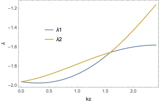
From the condition in the ConditionalExpression of the second root, the switchover occurs at

{so = Reduce[{sol[kz][[2, 1, -1, -1, 2]], 1 < kz < 2}, kz][[1, -1]], so // N}
(* {200/131 ArcTan[(33 Sqrt[3/23])/7], 1.58739} *)

EDIT: Alternatively, to find the switchover use

{so = kz /. 
   Solve[{Equal @@ (λ /. Most[sol[kz] // Normal]), 1 < kz < 2}, 
     kz][[1]], so // N}
(* {200/131 ArcTan[(33 Sqrt[3/23])/7], 1.58739} *)

Using Piecewise, the smooth curves are then

Format[lambda[n_]] = Subscript[λ, n];
lambda[1][kz_] = Piecewise[{
    {λ /. sol[kz][[1]], kz <= so},
    {λ /. sol[kz][[2]], so < kz < Pi/1.31}}];
lambda[2][kz_] = Piecewise[{
    {λ /. sol[kz][[2]], kz <= so},
    {λ /. sol[kz][[1]], so < kz < Pi/1.31}}];
Plot[{lambda[1][kz], lambda[2][kz]}, {kz, 0, Pi/1.31},
 Frame -> True,
 FrameLabel -> (Style[#, 12, Bold] & /@ {kz, λ}),
 PlotLegends -> Placed[{lambda[1], lambda[2]}, {.25, .6}]]

When the plots extend out farther to the right, the problem remains, no? — LouisB, Sep 07 '21 at 03:55
Yes. I used the plot range indicated in the OP's code, i.e., {kz, 0, Pi/3}. The smooth curves switch between branches of the solution. This is caused by meeting the conditions of the ConditionalExpressions. — Bob Hanlon, Sep 07 '21 at 04:52
@BobHanlon I made a mistake, the range of kz is from 0 to Pi/1.31. So LouisB is correct if you extend the plots, the two solutions switches. I made the necessary edits in the question. — sslucifer, Sep 07 '21 at 07:53

Aren't roots of polynomial equations smooth functions of their parameters?

2 Answers2

Linked