How can I shade specific regions between two curves in a Plot?

Question

From

Plot[{
  ((0.707106 Sqrt[1 - 1.5 s13^2] + 0.5 s13)^2)/(1 - s13^2), 
  ((0.707106 Sqrt[1 - 1.5 s13^2] - 0.5 s13)^2)/(1 - s13^2)}, 
  {s13, 0.0, 0.23},
  PlotRange -> {{0.0, 0.23}, {0.35, 0.67}}, Frame -> True,
  FrameLabel -> {FrameLabel -> {sin13, sin223}},
  PlotStyle -> {{Gray, Thick}, {Brown,Thick}},
  LabelStyle -> Directive[Black, Bold], Filling -> True,
  FillingStyle -> Directive[Opacity[.19], Green]
]

I obtained this

enter image description here

But I want to shade definite regions of the axes with different colors. Like

sorry for poor quality of the 2nd picture

You can try combining this Plot with a RegionPlot using Show. — Spawn1701D, May 23 '13 at 02:45

Michael E2 · Accepted Answer · 2013-05-23T11:53:07.130

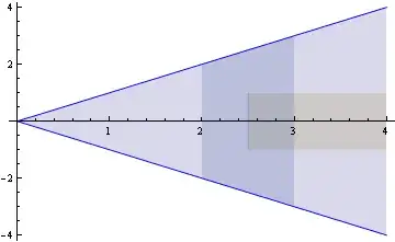
With ParametricPlot, you can use Mesh and its friends. The MeshShading is a matrix of colors that maps onto the grid created by the mesh. Here it's 3 x 4 color matrix. Apply ParametricPlot to {s13, f (1 - t) + g t} which interpolates between the two curves.

With[{f = ((0.707106 Sqrt[1 - 1.5 s13^2] + 0.5 s13)^2)/(1 - s13^2),
      g = ((0.707106 Sqrt[1 - 1.5 s13^2] - 0.5 s13)^2)/(1 - s13^2)}, 
 Show[
  ParametricPlot[
   {s13, f (1 - t) + g t}, {s13, 0.0, 0.23}, {t, 0, 1},
   PlotRange -> {{0.0, 0.23}, {0.35, 0.67}},
   MeshFunctions -> {#1 &, #2 &},  (* x, y *)
   Mesh -> {{0.04, 0.1, 0.15}, {0.46, 0.54}}, (* x, y coords *)
   MeshStyle -> None,
   MeshShading -> {
     {Directive[Opacity[.19], Green], Directive[Opacity[.19], Green],
       Green, Directive[Opacity[.19], Green]},
     {Directive[Opacity[.19], Green], Yellow, Brown, Yellow},
     {Directive[Opacity[.19], Green], Directive[Opacity[.19], Green],
       Green, Directive[Opacity[.19], Green]}},
   Frame -> True, FrameLabel -> {sin13, sin223},
   AspectRatio -> 1/GoldenRatio],
  Plot[{f, g}, {s13, 0.0, 0.23}, 
   PlotStyle -> {Directive[Gray, Thick], Directive[Brown, Thick]}]
  ]
 ]

Output

I had to add the boundary lines by hand using Plot, since there can be only a single BoundaryStyle.

(Edit notice: Originally, I goofed and made the boundary line straight lines.)

@BiswajitKarmakar You're welcome. Note the fix to the boundary lines. I was tired and carelessly made them straight -- and they looked right, but the fix will work with graphs that are more curved. — Michael E2, May 23 '13 at 11:55
@Micael E2, I noticed that (zooming the image in output of the code),thinking what's going on. I'm learning these ParametricPlot, Mesh etc. stuffs now. — Doon, May 23 '13 at 13:34

Dr. belisarius · Answer 2 · 2013-05-23T04:18:14.013

6

Perhaps something like:

Plot[{x, -x, 
       UnitStep[x - 2.5],   -UnitStep[x - 2.5], 
      x UnitBox[x - 2.5], - x UnitBox[x - 2.5]}, 
      {x, 0, 4}, 
      PlotStyle -> Join[Blue {1, 1}, ConstantArray[None, 4]],
      Filling -> {1 -> {2}, 3 -> {4}, 5 -> {6}}]

enter image description here

edited May 23 '13 at 04:18

answered May 23 '13 at 03:35

Dr. belisarius

115,881
13
203
453

thanks a lot for your suggestion. – Doon May 23 '13 at 05:24

kglr · Answer 3 · 2018-01-04T03:36:17.383

All can be done in a single ParametricPlot by adding #4& as the third mesh function with appropriate mesh values in @MichaelE2's answer:

With[{f = ((0.707106 Sqrt[1 - 1.5 s13^2] + 0.5 s13)^2)/(1 - s13^2), 
  g = ((0.707106 Sqrt[1 - 1.5 s13^2] - 0.5 s13)^2)/(1 - s13^2)}, 
 ParametricPlot[{s13, f (1 - t) + g t}, {s13, 0.0, 0.23}, {t, 0, 1}, 
  PlotRange -> {{0.0, 0.23}, {0.35, 0.67}}, 
  MeshFunctions -> {#1 &, #2 &, #4 &}, BoundaryStyle -> None, 
  MeshStyle -> Opacity[0], ImageSize -> 600, 
  Mesh -> {{0.04, 0.1, 0.15}, {0.46, 0.54},
   {{0, Directive[Thickness[.01], Opacity[1, Gray]]}, 
    {1, Directive[Thickness[.01], Opacity[1, Brown]]}}}, 
  MeshShading -> {{{Directive[Opacity[.19], Green], 
      Directive[Opacity[.19], Green], Green, Directive[Opacity[.19], Green]}, 
    {Directive[Opacity[.19], Green], Yellow, Brown, Yellow}}},
  Frame -> True, FrameLabel -> {sin13, sin223}, AspectRatio -> 1/GoldenRatio]]

How can I shade specific regions between two curves in a Plot?

3 Answers3

Linked