Double integral 0

Question

I am trying to reproduce the results from a paper in Mathematica. This task involves $K$ double integrals of the form

$$\int f(x,y)g(x)dx,$$

where $f(x,y)$ is a bivariate normal density with mean $(-4.08, -3.41)$ and diagonal covariance matrix with diagonal $(1/10,1/21)$, and $g(x)$ is a normal density with mean $\beta_0+\beta_1\xi$ and variance $\sigma_e^2$ (all of them known). I want to obtain this integral as a function of $\xi$.

Sigma = {{1/10, 0}, {0, 1/21}}

    {β0, β1, σe} = \
{-2.3, 0.5, 0.0005}



    f[ξ_] := 
 NIntegrate[
  PDF[MultinormalDistribution[{-4.08, -3.41}, Sigma], {η, ξ}]*
   PDF[NormalDistribution[β0 + β1*ξ, σe], \
η], {η, -∞, ∞}]

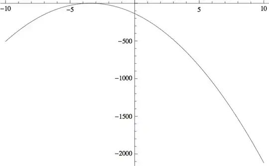
   Plot[f[t], {t, -10, 10}]

This code returns a $0$ for all values of $\xi$, while the true value should not be $0$.

How can I obtain this integral? What seems to be the problem? Is it the precision? Any ideas would be greatly appreciated.

My impression so far is that the $\sigma_e$ is very small and therefore the densities involved in the integration are very concentrated. This makes difficult the automatic integration.

@JonathanShock Thank you for pointing this out. I have defined these variables and included some explanation. — Roman, May 28 '13 at 23:14
Take a look at the function you are trying to integrate. It is enormously small. You will have to be extremely careful with the precision in this calculation. — Jonathan Shock, May 28 '13 at 23:17
@JonathanShock Indeed, I have included a comment on this (last paragraph). Maybe this is why the automatic integration (-Inf,Inf) is not identifying a proper integration range. — Roman, May 28 '13 at 23:19

score 4 · Accepted Answer · edited Aug 16 '13 at 12:44

4

The problem is the numerical precision that is required for this calculation.

Thankfully the integral can be performed analytically and then the plot can be created. It is actually easier perhaps in this case to create a ListPlot though you can do it with a LogPlot too:

f[ξ_]=Integrate[
PDF[MultinormalDistribution[{-4.08, -3.41}, Sigma], {η, ξ}]*PDF[NormalDistribution[β0 + β1*ξ, σe], \
η], {η, -∞, ∞}]
{#, Log[f[#]]} & /@ Range[-10, 10, 0.1];
ListLinePlot[%]

Result of integral

edited Aug 16 '13 at 12:44

M6299

1,471
1
13
20

answered May 28 '13 at 23:30

Jonathan Shock

3,015
15
24

Many thanks. You have wisely noticed that the integral can be obtained in closed form. I was comparing my own calculations with the numerical integral and then I came across this issue. – Roman May 28 '13 at 23:33
Update: The range of interest for $f$ is around $(-4.5,-2.5)$. In this range there is no need to use the $\log$. – Roman May 28 '13 at 23:56
Indeed, this is true. – Jonathan Shock May 29 '13 at 00:16
Jonathan, your alternative interpretation of a recently deleted question was addressed here: http://mathematica.stackexchange.com/q/7836/121 – Mr.Wizard May 29 '13 at 02:24
@Mr.Wizard, many thanks. – Jonathan Shock May 29 '13 at 02:28

Double integral 0

1 Answers1