Integro-differential equation with double integral

Question

I am looking at the following variation of a integro-differential, with y[0]=1. The output is not great, any solutions to this?

Clear[s, t, J, w];
J[w_] := 1/(2 + w^2)
eqn = y'[t] == -Integrate[y[t1] J[w] Exp[I (0.1 - w) (t1 - t)], {w, 0, ∞}, {t1, 0,t}]
LaplaceTransform[eqn, t, s]
InverseLaplaceTransform[%, s, t]
ySol[t_] = y[t] /. First[%] /. y[0] -> 1
Plot[ySol[t], {t, 0, 10}, PlotRange -> {-1, 1}]

Update:

I received some feedback from a Wolfram Support Engineer regarding this question — it appears that current versions of Mathematica are unable to solve this sort of integro-differential equations. Hopefully we will be able to see better implementations and future versions can crack this sort of equations.

I guess you're trying to use the method I posted here, but the first thing one needs to correct then is that you have to say Solve[%, LaplaceTransform[y[t], t, s]] before doing InverseLaplaceTransform[%, s, t]. That's not the real problem, though. Since you have two integrals, the solution would involve two Laplace transforms. Note that the w integral is itself a Laplace transform integral. — Jens, May 31 '13 at 05:35
That's exactly right, this prob. is an extension of the earlier one, however you may note that the integrand involving J(w) can be sorted out at the earlier stage, and then you ony have to deal with one laplace transform? — thils, May 31 '13 at 05:47
Come to think of it, I may not be right as the inner inregrant is dependent on y.... — thils, May 31 '13 at 05:56
Yes, it's not so simple. One can simplify things with a translation of the t variables, but I'm out of time for today. — Jens, May 31 '13 at 06:05
I get this output: "Unable to prove that integration limits {0,t} are real. Adding
assumptions may help" — thils, May 31 '13 at 06:54
As a note, you do not need to nest Integrate, it accepts multiple limits. See the third form in the docs. — rcollyer, May 31 '13 at 13:02
Yes, there appears to be improvement when I use the nest (edited the input now), but output still not great. The bigger issue is what happens if there is no analytical solution, does NIntegrate needs to be used? — thils, May 31 '13 at 18:32

score 2 · Answer 1 · answered Feb 09 '24 at 12:27

This problem can be solved with the Euler wavelets collocation method even in v.8 as follows

J[w_] := 1/(2 + w^2)
eqn = y'[
   t] == -Integrate[
    y[t1]  J[w]  Exp[I  (0.1 - w)  (t1 - t)], {w, 
     0, \[Infinity]}, {t1, 0, t}]

First step. Let define kernel by integration on w

Integrate[
 Exp[I  (-1/10 + w)  dt]/(2 + w^2), {w, 0, \[Infinity]}, 
 Assumptions -> {dt > 0}]
(Out[]= (E^(-((I dt)/
  10)) (E^(-Sqrt[2] dt) [Pi] + 
   I Sqrt[[Pi]]
     MeijerG[{{1/2}, {}}, {{1/2, 1/2}, {0}}, dt^2/2]))/(2 Sqrt[2]))

Therefore

kernel[dt_] := (
 E^(-((I dt)/
   10)) (E^(-Sqrt[2] dt) \[Pi] + 
    I Sqrt[\[Pi]] MeijerG[{{1/2}, {}}, {{1/2, 1/2}, {0}}, dt^2/2]))/(
 2 Sqrt[2])

Second step. Using kernel and substitution t1 = t s we transform equation into Fredholm type

eqn = {y'[t] + t  NIntegrate[kernel[t - t  s] y[t  s], {s, 0, 1}] == 
   0, y[0] == 1};

Third step. Let define y[t],D[y[t],t] in the Euler wavelets base as

UE[m_, t_] := EulerE[m, t];
psi[k_, n_, m_, t_] := 
  Piecewise[{{2^(k/2)   UE[m, 2^k  t - 2  n + 1], (n - 1)/2^(k - 1) <=
       t < n/2^(k - 1)}, {0, True}}];
PsiE[k_, M_, t_] := 
 Flatten[Table[psi[k, n, m, t], {n, 1, 2^(k - 1)}, {m, 0, M - 1}]]
k0 = 3; M0 = 4; With[{k = k0, M = M0}, 
 nn = Length[Flatten[Table[1, {n, 1, 2^(k - 1)}, {m, 0, M - 1}]]]];
dx = 1/(nn); xl = Table[l*dx, {l, 0, nn}]; xcol = 
 Table[(xl[[l - 1]] + xl[[l]])/2, {l, 2, nn + 1}]; Psijk = 
 With[{k = k0, M = M0}, PsiE[k, M, t1]]; Int1 = 
 With[{k = k0, M = M0}, Integrate[PsiE[k, M, t1], t1]]; 
Psi[y_] := Psijk /. t1 -> y; 
int1[y_] := Int1 /. t1 -> y; vary = Array[yy, {nn}]; 
y[t_] := vary . int1[t] + b0 ; dy[t_] := vary . Psi[t];

Final step. We define system of linear equations and solve it using LinearSolve

int2 = Table[
  t  NIntegrate[kernel[t - t  s] int1[t  s], {s, 0, 1}], {t, xcol}];
int0 = Table[t  NIntegrate[kernel[t - t  s], {s, 0, 1}], {t, xcol}];
eqs = Join[
   Table[vary . Psi[xcol[[i]]] + vary . int2[[i]] + b0  int0[[i]] == 
     0, {i, nn}], {y[0] == 1}];
var = Join[vary, {b0}]; {vec, mat} = CoefficientArrays[eqs, var];
sol = LinearSolve[mat, -vec];

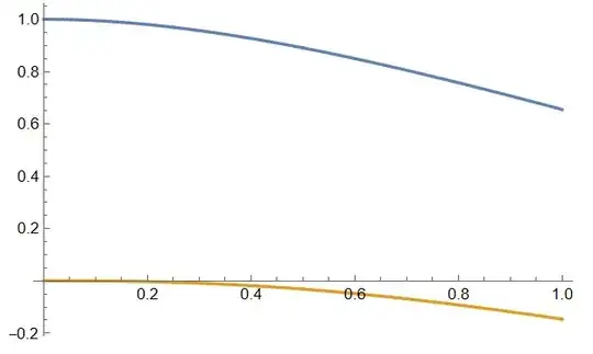
Visualization

rule = Table[var[[i]] -> sol[[i]], {i, Length[var]}]; Plot[
 Evaluate[ReIm[y[t] /. rule]], {t, 0, 1}]

Interesting answer. Shouldn't the assumption be dt<0 in the calculation of the kernel? — Ulrich Neumann, Feb 10 '24 at 13:55
Please, pay attention that I used Exp[I (-1/10 + w) dt]/(2 + w^2) while in the eqn there is opposite sine in exp as J[w] Exp[I (0.1 - w) (t1 - t)], therefore dt=t-t1>0. — Alex Trounev, Feb 10 '24 at 14:43

Integro-differential equation with double integral

Update:

1 Answers1