NIntegrate giving different results after a change of variables

Question

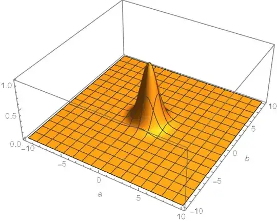
When I compute numerically the following double integral: \begin{equation} f(x,y)=\int_{-\infty}^{+\infty}da\int_{-\infty}^{+\infty}db\, \cosh\left[\frac{\sinh^{-1}(a)-\sinh^{-1}(b)}{2}\right]\, \exp\left\{-\frac{a^2+b^2}{2}\right\}\\ \cos\bigg[x\,(a-b)+y\,(\sqrt{1+a^2}-\sqrt{1+b^2}) \bigg] \end{equation} I get:

In[1]:= f[x_,y_] := NIntegrate[Cosh[(ArcSinh[a]-ArcSinh[b])/2]*Exp[-1/2*(a^2+b^2)]*Cos[x*(a-b)+y*Sqrt[1+a^2]-Sqrt[1+b^2])], {a,-Infinity,+Infinity}, {b,-Infinity,+Infinity}];
In[2]:= f[20, 10]
NIntegrate::slwcon: Numerical integration converging too slowly; suspect one of the following: singularity, value of the integration is 0, highly oscillatory integrand, or WorkingPrecision too small.
NIntegrate::eincr: The global error of the strategy GlobalAdaptive has increased more than 2000 times. The global error is expected to decrease monotonically after a number of integrand evaluations. Suspect one of the following: the working precision is insufficient for the specified precision goal; the integrand is highly oscillatory or it is not a (piecewise) smooth function; or the true value of the integral is 0. Increasing the value of the GlobalAdaptive option MaxErrorIncreases might lead to a convergent numerical integration. NIntegrate obtained -1.4135310^-15 and 5.954955635986372`^-12 for the integral and error estimates.
Out[2]:= -1.41353*10^-15

While under the change of variables $a=\sinh(\alpha)$, $b=\sinh(\beta)$ the integral becomes: \begin{equation} f(x,y)=\int_{-\infty}^{+\infty}d\alpha\int_{-\infty}^{+\infty}d\beta\, \cosh(\alpha)\,\cosh(\beta)\,\cosh\left(\frac{\alpha-\beta}{2}\right)\\ \exp\left\{-\frac{\sinh^2(\alpha)+\sinh^2(\beta)}{2} \right\}\\ \cos\bigg[x\,\left[\sinh(\alpha)-\sinh(\beta)\right]+y\,\left[\cosh(\alpha)-\cosh(\beta)\right] \bigg] \end{equation} and the result changes as:

In[1]:= f[x_,y_] := NIntegrate[Cosh[α]*Cosh[β]*Cosh[(α-β)/2]*Exp[-1/2*((Sinh[α])^2+(Sinh[β]])^2)]*Cos[x*(Sinh[α]-Sinh[β])+y*(Cosh[α]-Cosh[β])], {α,-Infinity,+Infinity}, {β,-Infinity,+Infinity}];
In[2]:= f[20, 10]
NIntegrate::levtime: Time spent solving linear system in LevinRule exceeded 10.seconds. Try increasing the value of the "TimeConstraint" option or decreasing the value of the "Points" option. NIntegrate::mtdfb: Numerical integration with LevinRule failed. The integration continues with Method -> MultiDimensionalRule. ... NIntegrate::eincr: The global error of the strategy GlobalAdaptive has increased more than 2000 times. The global error is expected to decrease monotonically after a number of integrand evaluations. Suspect one of the following: the working precision is insufficient for the specified precision goal; the integrand is highly oscillatory or it is not a (piecewise) smooth function; or the true value of the integral is 0. Increasing the value of the GlobalAdaptive option MaxErrorIncreases might lead to a convergent numerical integration. NIntegrate obtained 8.208407293650954*^-9 and 0.000016005954816250418` for the integral and error estimates.
Out[2]:= 8.20841*10^-9

Why the two results are different? How can I improve the numerical computation?

Answer 1

Both results indicate the both integrals result in zero.

The integrand is dominated by the part Cosh[(ArcSinh[a] - ArcSinh[b])/2]*Exp[-1/2*(a^2 + b^2)]

Plot3D[ Cosh[(ArcSinh[a] - ArcSinh[b])/2]*Exp[-1/2*(a^2 + b^2)] 
, {a, -10 , +10 }, {b, -10 , +10 }, 
PlotPoints -> 100, PlotRange -> All, AxesLabel -> {a, b}] 

For numerical reasons it is sufficient to decrease the integration range accordingly.

inf=10; 
f[x_, y_] :=NIntegrate[
Cosh[(ArcSinh[a] - ArcSinh[b])/2]*Exp[-1/2*(a^2 + b^2)]*
Cos[x*(a - b) +y*(Sqrt[1 + a^2] -Sqrt[1 + b^2])], {a, -inf, +inf}, {b, -inf, +inf}, Method -> "LocalAdaptive" , 
IntegrationMonitor :> ((errors = Through[#1@"Error"]) &)];
f[20, 10 ]   (* result 1.8670410^-45)
Total@errors  (* error 1.9367410^-46)

Hope it helps!