Manual Runge-Kutta 2 for a system of 4 ODE's

Question

I have the following system:

$\frac{dx}{dt} = p_x \\ \frac{dy}{dt} = p_y \\ \frac{dp_x}{dt}=-\frac{\partial V}{\partial x} \\ \frac{dp_y}{dt}=-\frac{\partial V}{\partial y}$

,where $V(x,y) = \frac{1}{2} (\omega_x x^2 + \omega_y y^2)$, and $\omega_x = 1, \omega_y = 2$. Following the advice in the linked page, I wrote the system in vector form, and now I would like to manually run a Do loop in order to solve it with a Runge-Kutta 2 method. The loop itself isn't difficult, and before the loop are the initial data

tf=100;
dt=1/10;
T=Table[i,{i,ti,tf,dt}];
X=ConstantArray[0,Length[T]];
Y=ConstantArray[0,Length[T]];
PX=ConstantArray[0,Length[T]];
PY=ConstantArray[0,Length[T]];
PX[[1]]=1;
PY[[1]]=1;
Do[k1=dt*f[T[[n]],X[[n]],Y[[n]],PX[[n]],PY[[n]]];
l1=dt*g[T[[n]],X[[n]],Y[[n]],PX[[n]],PY[[n]]];
m1=dt*h[T[[n]],X[[n]],Y[[n]],PX[[n]],PY[[n]]];
n1=dt*p[T[[n]],X[[n]],Y[[n]],PX[[n]],PY[[n]]];
k2=dt*f[(T[[n]]+dt/2),(X[[n]]+k1/2),(Y[[n]]+l1/2),(PX[[n]]+m1/2),(PY[[n]]+n1/2)];
l2=dt*g[(T[[n]]+dt/2),(X[[n]]+k1/2),(Y[[n]]+l1/2),(PX[[n]]+m1/2),(PY[[n]]+n1/2)];
m2=dt*h[(T[[n]]+dt/2),(X[[n]]+k1/2),(Y[[n]]+l1/2),(PX[[n]]+m1/2),(PY[[n]]+n1/2)];
n2=dt*p[(T[[n]]+dt/2),(X[[n]]+k1/2),(Y[[n]]+l1/2),(PX[[n]]+m1/2),(PY[[n]]+n1/2)];
X[[n+1]]=X[[n]]+k2;
Y[[n+1]]=Y[[n]]+l2;
PX[[n+1]]=PX[[n]]+m2;
PX[[n+1]]=PY[[n]]+n2, {n,1, Length[X]-1}]

However, I'm having trouble understanding how to apply the code to my vector of equations: How should I define the functions $f,g,h$ and $p$?

Edit: Thanks to everyone who contributed. I also came up with a simple solution to define the function in vector form, which also shortens the code considerably, so I'm uploading it for anyone who might be interested:

n1=1000;
h=0.1;
T=Table[i,{i,0,100,h}];
F[t_,{x_,y_,px_,py_}]:={px,py,-x,-2*y};
U=ConstantArray[{0.,0.,1.,1.},n1+1];
Do[K1=hF[T[[i]],U[[i]]];

K2=hF[T[[i]]+h/2,U[[i]]+K1/2];
U[[i+1]]=U[[i]]+K2,
{i,1,n1}]
X=U[[All,1]];
Y=U[[All,2]];
PX=U[[All,3]];
PY=U[[All,4]];
ListPlot[Transpose[{T,X}],PlotLabel->"x(t)",AxesLabel->{"t","x"}]
ListPlot[Transpose[{T,Y}],PlotLabel->"y(t)",AxesLabel->{"t","y"}]
energy=(PX^2 + PY^2)/2 + (X^2 + 2*(Y^2))/2;
ListPlot[Transpose[{T,energy}],PlotLabel->"Energy",AxesLabel->{"t","E(t)"}]
ListPlot[Transpose[{T,energy-energy[[1]]}],PlotLabel->"Energy error",AxesLabel->{"t","E(t)-E(0)"}]

Alex Trounev · Accepted Answer · 2022-01-17T04:33:34.970

Using JBuck's code with implementation the midpoint method of rk2 family we have

Clear["Global`*"]
V = 1/2 (x1^2 + 2 y1^2);
ti = 0; tf = 10;
dt = 1./10;
T = Table[i, {i, ti, tf, dt}];
X = ConstantArray[0, Length[T]];
Y = ConstantArray[0, Length[T]];
PX = ConstantArray[0, Length[T]];
PY = ConstantArray[0, Length[T]];
PX[[1]] = 1;
PY[[1]] = 1;
f[t_, x_, y_, px_, py_] := px; g[t_, x_, y_, px_, py_] := py; 
h[t_, x_, y_, px_, py_] := -D[V, x1] /. {x1 -> x, y1 -> y}; 
p[t_, x_, y_, px_, py_] := -D[V, y1] /. {x1 -> x, y1 -> y};
Do[k1 = dt f[T[[n]], X[[n]], Y[[n]], PX[[n]], PY[[n]]];
 l1 = dt g[T[[n]], X[[n]], Y[[n]], PX[[n]], PY[[n]]];
 m1 = dt h[T[[n]], X[[n]], Y[[n]], PX[[n]], PY[[n]]];
 n1 = dt p[T[[n]], X[[n]], Y[[n]], PX[[n]], PY[[n]]];
 k2 = dt f[T[[n]] + dt/2, X[[n]] + k1/2, Y[[n]] + l1/2, 
    PX[[n]] + m1/2, PY[[n]] + n1/2];
 l2 = dt g[T[[n]] + dt/2, X[[n]] + k1/2, Y[[n]] + l1/2, 
    PX[[n]] + m1/2, PY[[n]] + n1/2];
 m2 = dt h[T[[n]] + dt/2, X[[n]] + k1/2, Y[[n]] + l1/2, 
    PX[[n]] + m1/2, PY[[n]] + n1/2];
 n2 = dt p[T[[n]] + dt/2, X[[n]] + k1/2, Y[[n]] + l1/2, 
    PX[[n]] + m1/2, PY[[n]] + n1/2];
 X[[n + 1]] = X[[n]] + k2;
 Y[[n + 1]] = Y[[n]] + l2;
 PX[[n + 1]] = PX[[n]] + m2;
 PY[[n + 1]] = PY[[n]] + n2;, {n, 1, Length[T] - 1}]

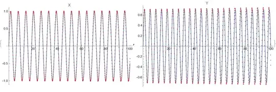
Visualization of numerical solution (red points) with NDSolve solution (solid lines)

sol = NDSolve[{x''[t] == -D[V, x1] /. {x1 -> x[t], y1 -> y[t]}, 
   y''[t] == -D[V, y1] /. {x1 -> x[t], y1 -> y[t]}, x[0] == 0, 
   y[0] == 0, x'[0] == 1, y'[0] == 1}, {x, y}, {t, ti, tf}];
{Show[Plot[x[t] /. sol[[1]], {t, ti, tf}, PlotLabel -> "X", 
   AxesLabel -> Automatic], 
  ListPlot[Transpose[{T, X}], PlotRange -> All, PlotStyle -> Red]], 
 Show[Plot[y[t] /. sol[[1]], {t, ti, tf}, PlotLabel -> "Y", 
   AxesLabel -> Automatic], 
  ListPlot[Transpose[{T, Y}], PlotRange -> All, PlotStyle -> Red]]}

Update 1. We can organize rk2 step in separate module as follows

Clear["Global`*"]
U = 1/2 (x1^2 + 2 x2^2); x = ConstantArray[0, 4]; 
f[t_, x_] := {x[[3]], 
  x[[4]], -D[U, x1] /. {x1 -> x[[1]], 
    x2 -> x[[2]]}, -D[U, x2] /. {x1 -> x[[1]], x2 -> x[[2]]}};
rk2[f_, h_][{t_, x_}] := Module[{k1, k2}, k1 = f[t, x];
  k2 = f[t + h/2, x + h k1/2];
  {t + h, x + h k2}]

We can use NestList instead of Do loop and compare numerical solution with NDSolve as well

tf = 100; dt = 1/10; sol = 
 NestList[rk2[f, dt], {0, {0, 0, 1, 1}}, Round[tf/dt]];
sol1 = NDSolve[{X''[T] == -D[U, x1] /. {x1 -> X[T], x2 -> Y[T]}, 
   Y''[T] == -D[U, x2] /. {x1 -> X[T], x2 -> Y[T]}, X[0] == 0, 
   Y[0] == 0, X'[0] == 1, Y'[0] == 1}, {X, Y}, {T, 0, tf}]; {Show[
  Plot[X[T] /. sol1[[1]], {T, 0, tf}, PlotLabel -> "X"], 
  ListPlot[Transpose[{sol[[All, 1]], sol[[All, 2, 1]]}], 
   PlotStyle -> Red]], 
 Show[Plot[Y[T] /. sol1[[1]], {T, 0, tf}, PlotLabel -> "Y"], 
  ListPlot[Transpose[{sol[[All, 1]], sol[[All, 2, 2]]}], 
   PlotStyle -> Red]]}

Every year thousands of students around the world get assignments to implement RK methods in MA. Then numerous questions appear here. What is really a pity that profs and course instructors delegate their direct duties to SE, and do not explain properly efficient programming strategies. I really cannot penetrate, why vectorized form is so opposed. What can be compactly written in a vector form is expanded to many lines. I am sure if there were 1000 equations students would still write a program with 2000+ lines. This is not a criticism of your post, in fact your answers are always so helpful. — yarchik, Jan 16 '22 at 13:00
@yarchik Thank you for your comment. I am also don't understand why not to organize code with rk method implemented in general as Module. Probably this is specific approach based on some student experience. — Alex Trounev, Jan 16 '22 at 13:34
I like your updated solution even more. There, you have just a small module where the RK2 logic is implemented. — yarchik, Jan 17 '22 at 09:07
I thought we can implement the trapezium rule, to conserve the energy of the system: $\vec{u_{n+1}} - \vec{u_n}=\frac{dt}{2}(\vec{f_{n+1}} + \vec{f_n})$, where $\vec{u}={x,y,p_x,p_y}, \frac{d \vec{u}}{dt}=\vec{f}(t, \vec{u})$, but I cannot see how the Do loop would have to change, maybe you have an idea? — JBuck, Jan 24 '22 at 02:01
@JBuck Do you mean Verlet integration like in this post https://mathematica.stackexchange.com/questions/208590/numerically-solving-a-system-of-many-coupled-non-linear-odes-efficiently ? — Alex Trounev, Jan 24 '22 at 02:32
I thought that, to obtain the future values of the momentum and position, we may use a Do loop at each time step, which can use a RK1 or RK2 step as initial guess, and then iterate the above system of equations 10 times, repeatedly substituting the last value $\vec{u}{n+1}$ into the function $\vec{f}{n+1}=\vec{f}(t_{n+1},\vec{u}{n+1})$ on the right hand side, to compute the new value of the LHS. That is, at each time step, we can perform an iteration $\vec{u}^{new}{n+1}=\vec{u}n+\frac{dt}{2}[\vec{f}(t{n+1},\vec{u}^{old}_{n+1})+\vec{f}(t_n, \vec{u}_n)]$ and stop after 10 iterations. — JBuck, Jan 24 '22 at 16:53
@JBuck What do you try to compute with iterations? As method of integration we use predictor-corrector. It starts from Euler step. — Alex Trounev, Jan 24 '22 at 17:23
@AlexTrounev right I see, my idea was probably inspired by something else, but couldn't be implemented here. — JBuck, Jan 24 '22 at 20:16

Manual Runge-Kutta 2 for a system of 4 ODE's

1 Answers1

Linked