Using FindRoot in a Loop: Updating the value of starting point

Question

Consider the following nonlinear equation for $h[\lambda]$

\[Beta] = 4.1; \[Kappa] = 
 50 \[Beta]; lb0 = 10; ug = 30; kg = 10^-2 ; kb = 5; n = 50;
B1 = Sqrt[([Sigma]1 + Sqrt[[Sigma]1^2 - 4 kg [Kappa]])/(
 2 [Kappa])]; B2 = Sqrt[([Sigma]1 - 
  Sqrt[[Sigma]1^2 - 4 kg [Kappa]])/(2 [Kappa])];
c[ [Lambda]_] := (ug - 1)/((2 [Pi] kg)/kb (1/B2^2 - 1/B1^2) + 
     1/2 Log[B1/B2] - 2 !(
*UnderoverscriptBox[([Sum]), (j = 1), (n)]((BesselK[*
StyleBox["0", "TI"], B1\ j\ [Lambda]\ ] - BesselK[*
StyleBox["0", "TI"], \ B2\ j\ [Lambda]\ ]))));
H[ [Lambda]_] := [Pi] c[ [Lambda]] kg (1/B2^2 - 1/B1^2) (n (ug - 1))
h[[Lambda]_] := D[H[ [Lambda]], [Lambda]]

The goal is to solve $h[\lambda]=0$ for different values of $\sigma1$. For example, for $\sigma1=0.08$ (assuming 50 as the start point)

\[Sigma]1 = 0.08;
FindRoot[h[\[Lambda]] == 0, {\[Lambda], 50}]
\[Sigma][1] = \[Sigma]1; \[Lambda]1[1] = Re[\[Lambda]] /. %;

which yields $\lambda=59.9638$. Now I want to increase the value of $\sigma1$ to 0.09 and use the root obtained for $\sigma1=0.08$ as the starting point to solve the new $h[\lambda]=0$ and continue doing it for $\sigma1=0.08, 0.09, 0.1, 0.11, ...$ and record the values of $\lambda1[1],\lambda1[2], ...$ for $\sigma1[1], \sigma1[2], ...$. For that, I need to make a loop that includes FindRoot and update the value of starting points anytime $h[\lambda]=0$ is solved for a given $\sigma1$. In other words, the starting point to find $\lambda1[i]$ for $\sigma1[i]$ must be $\lambda1[i-1]$ obtained for $\sigma1[i-1]$. How can I do that?

closely related/possible duplicate Q/As: (1) Backsubstituting solution into FindRoot and (2) Using previous two solutions as a start point in FindRoot — kglr, Feb 02 '22 at 01:40

Bob Hanlon · Answer 1 · 2022-02-02T03:12:04.690

Clear["Global`*"]

β = 41/10; 
κ = 50 β; 
lb0 = 10; 
ug = 30; 
kg = 10^-2 ; 
kb = 5; 
n = 50;

B1 = Sqrt[(σ1 + Sqrt[σ1^2 - 4 kg κ])/(2 κ)];
B2 = Sqrt[(σ1 - Sqrt[σ1^2 - 4 kg κ])/(2 κ)];

c[λ_] := (ug - 1)/(((2*Pi*kg)/kb)*(1/B2^2 - 1/B1^2) + 
     (1/2)*Log[B1/B2] - 
          2*Sum[BesselK[0, B1*j*λ] - BesselK[0, B2*j*λ], 
              {j, 1, n}]); 

H[ λ_] := π c[λ] kg (1/B2^2 - 1/B1^2) (n (ug - 1));

h[λ_] := D[H[λ], λ];

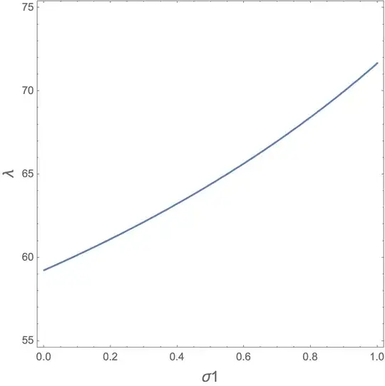
A ContourPlot of h[λ] == 0 provides a simple linear estimate of λ as a function of σ1

conPlt = ContourPlot[Evaluate[h[λ] == 0],
  {σ1, 0, 1}, {λ, 55, 75},
  FrameLabel -> (Style[#, 14] & /@ {σ1, λ})]

lambda[s_?NumericQ] :=
  Module[{sp = SetPrecision[s, 15]},
   λ /. FindRoot[h[λ] == 0 /. σ1 -> s, {λ, 12 (sp + 5)},
    WorkingPrecision -> 15]] // Quiet

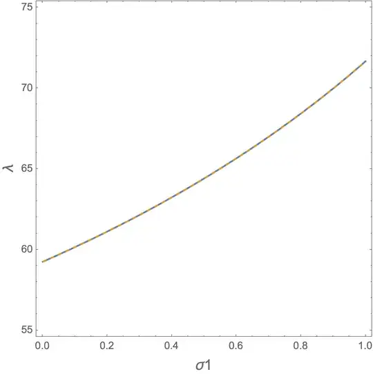
Comparing a plot of lambda with the ContourPlot to verify that lambda accurately tracks λ

Show[conPlt,
  Plot[lambda[σ1], {σ1, 0, 1},
   PlotStyle -> Directive[ColorData[97][2], Dashed]]] // Quiet

score 1 · Accepted Answer · answered Feb 02 '22 at 11:54

You can do this using "NestList":

We start with {0.08, 50} where the first value is sigma and the second the starting value. Then we define a function {#[[1]] + 0.01, λ /. FindRoot[h[λ] == 0 /. σ1 -> #[[1]], {λ, #[[2]]}] // Chop} & that calculates the next starting value and the current root. "NestList" will repeat this n times:

σ1 =.;
n=5; (* how many time to repeat*)
res = NestList[{#[[1]] +  0.01, λ /. 
       FindRoot[h[λ] == 0 /. σ1 -> #[[1]], {λ, #[[2]]}] // 
      Chop} &, {0.08, 50}, n];

Now in "res" we have the next starting value and the current root. Therefore we must correct for this:

res=Transpose[{Most[res[[All, 1]]], Rest[res[[All, 2]]]}]

Using FindRoot in a Loop: Updating the value of starting point

2 Answers2