How to make all the balls move until they stop by NBodySimulation

Question

n = 4;
countTime = 5;
SeedRandom[5];
initPos = RandomPoint[Disk[], n];
data = NBodySimulation[
   Association["PairwisePotential" -> "Coulomb", "Region" -> Disk[], 
    "ExternalForce" -> (Quantity[-0.5 Normalize[
          QuantityMagnitude[#["Velocity"]]](*An extra damping*), "Newtons"] &)], <|
      "Mass" -> Quantity[1, "Kilograms"], 
      "Position" -> Quantity[#, "Meters"], 
      "Velocity" -> Quantity[{0, 0}, "Meters"/"Seconds"], 
      "Charge" -> Quantity[10^-5, "Coulombs"]|> & /@ initPos, 
   countTime];
colors = RandomColor[n];
Manipulate[
 Graphics[{Circle[], Red, PointSize[0.02], 
   Riffle[colors, Point /@ data[All, "Position", time]]}, 
  Axes -> True], {time, $MachineEpsilon, countTime, 
  Appearance -> "Labeled"}]

I noticed that because one of the balls is coming to rest, the other balls can no longer be simulated because the iteration spacing is 0 after t>4.09486. How can I solve this problem so that the simulation continues until all the balls are at rest?

I guess we can change certain system options by Block? But I don't know which system option is causing this error...

You can control the method of integration for the underlying NDSolve by providing the option Method. Because the systems are Hamiltonian, the default choice in NBodySimulation is "SymplecticPartitionedRungeKutta". You can try with Method -> "StiffnessSwitching" which goes past the stiffness point, but soon after that, unfortunately, the balls wander outside the circle ... Internally, reflections from the walls are performed via WhenEvents. Perhaps there is already an answer here at MMA.SE on how to properly set up WhenEvents for such cases ... — Domen, Feb 24 '22 at 19:50
@Domen I note the method of ExplicitMidpoint ,StiffnessSwitching and Extrapolation all will avoid error result the balls wander outside the circle. I don't know if this is a bug or not in NBodySimulation — yode, Feb 24 '22 at 20:24
@yode What force do you try to describe with option "ExternalForce" -> (Quantity[-0.5 Normalize[ QuantityMagnitude[#["Velocity"]]](*An extra damping*), "Newtons"] &)? — Alex Trounev, Feb 25 '22 at 05:07
@AlexTrounev If I don't add damping to the charge, those charges will never stop. This force I am describing is like friction, always in the opposite direction to the speed and constant in magnitude. — yode, Feb 25 '22 at 05:41

Alex Trounev · Answer 1 · 2022-02-25T23:21:16.577

If we put countTime = 20 and remove Normalize then we have desired rest state

n = 4;
countTime = 20;
SeedRandom[5];
initPos = RandomPoint[Disk[], n];
data = NBodySimulation[
   Association["PairwisePotential" -> "Coulomb", "Region" -> Disk[], 
    "ExternalForce" -> (Quantity[-0.5 QuantityMagnitude[#[
           "Velocity"]](*An extra damping*), "Newtons"] &)], <|
      "Mass" -> Quantity[1, "Kilograms"], 
      "Position" -> Quantity[#, "Meters"], 
      "Velocity" -> Quantity[{0, 0}, "Meters"/"Seconds"], 
      "Charge" -> Quantity[10^-5, "Coulombs"]|> & /@ initPos, 
   countTime];
colors = RandomColor[n];
Manipulate[
 Graphics[{Circle[], Red, PointSize[0.02], 
   Riffle[colors, Point /@ data[All, "Position", time]]}, 
  Axes -> True], {time, $MachineEpsilon, countTime, 
  Appearance -> "Labeled"}]

We also can regularized force proposed by yode as follows

n = 4;
countTime = 8;
SeedRandom[5];
initPos = RandomPoint[Disk[], n];
data = NBodySimulation[
   Association["PairwisePotential" -> "Coulomb", "Region" -> Disk[], 
    "ExternalForce" -> (Quantity[-.5 (1 - 
           Exp[-10 Norm[QuantityMagnitude[#["Velocity"]]]]) Normalize[
          QuantityMagnitude[#["Velocity"]]](*An extra damping*), 
        "Newtons"] &)], <|"Mass" -> Quantity[1, "Kilograms"], 
      "Position" -> Quantity[#, "Meters"], 
      "Velocity" -> Quantity[{1. 10^-12, 0}, "Meters"/"Seconds"], 
      "Charge" -> Quantity[10^-5, "Coulombs"]|> & /@ initPos, 
   countTime];
colors = RandomColor[n];
Manipulate[
 Graphics[{Circle[], Red, PointSize[0.02], 
   Riffle[colors, Point /@ data[All, "Position", time]]}, 
  Axes -> True], {time, $MachineEpsilon, countTime, 
  Appearance -> "Labeled"}]

Hi, if we remove Normalize that means that the faster the ball is, the more damped it is, which is probably not a physical reality. The damping should be velocity independent. — yode, Feb 25 '22 at 09:47
@yode Actually damping is velocity dependent, for instance, in the water or air the friction force is proportional to $-k\vec{v}$ at small v and $-k_1|v|\vec{v}$ at large v. — Alex Trounev, Feb 25 '22 at 09:59
Well, I mean in a disc that ignores air resistance as this post. :) — yode, Feb 25 '22 at 10:02
@yode Do you try to describe dry friction with some minimal velocity to start? — Alex Trounev, Feb 25 '22 at 10:09
@yode I see, that for this specific unphysical force $−0.5\vec{v} /v$ there is unphysical result. :) But with regularized force $−0.5(1-e^{10 v})\vec{v} /v$ we have desired rest state - see update to my answer. — Alex Trounev, Feb 25 '22 at 23:24

xzczd · Accepted Answer · 2022-02-25T14:17:00.010

Solution 1

Funny, I'm not sure if this is the only solution, but Method -> "ExplicitEuler" (we know this is a rather primary method for ODE solving) solves the problem. This seems to be the first time I found a problem can be resolved with ExplicitEuler!

I've also added StartingStepSize -> 10^-3 to speed up the calculation a bit. (The default step choosing is around 10^-6, which turns out to be unnecessarily small. ) The calculation takes about 6 seconds on my laptop, tested in v12.3.1.

Result:

ListPlot[#, PlotRange -> All] & /@ data[All, "Position"]

Mathematica graphics

Solution 2

Not as straightforward and efficient as Solution 1, but a possible work-around is to define a smoother Normalize:

norm = Compile[{{v, _Real, 1}}, 
  If[v == {0, 0}, {0., 0.}, 2/Pi ArcTan[10^4 Total[v^2]] v/Sqrt@Total[v^2]], 
  RuntimeOptions -> EvaluateSymbolically -> False]

Use norm instead of Normalize in the code produces a solution visually the same as that of Solution 1, it takes about 26 seconds on my laptop, though.

Remark

I attempted to spot the root of problem, without success. But NBodySimulation has probably set up the system properly, because even if the problem is set up with NDSolve and WhenEvent manually, the issue remains.

The following is the code. Definition of data is the same as that of OP, definition of reflect is taken from this post, showStatus is from this post:

reflect[vector_, normal_] = -(vector - 2 (vector - Projection[vector, normal]));
f[x_, y_] = x^2 + y^2 - 1;
eq = data["Equations"] /. {Subscript[[FormalQ], i_] :> Subscript[x, i], 
    Subscript[[FormalP], i_] :> Subscript[x, i]', [FormalT] -> t};
event = WhenEvent[
     f @@ #[t] == 
      0, {#'[t] -> 
       reflect[#'[t], {Derivative[1, 0][f] @@ #[t], 
         Derivative[0, 1][f] @@ #[t]}]}] & /@ (Subscript[x, #] & /@ Range[4]);
var = (Subscript[x, #] & /@ Range[4])[t] // Through;
init = <|"Mass" -> Quantity[1, "Kilograms"], "Position" -> Quantity[#, "Meters"], 
     "Velocity" -> Quantity[{0, 0}, "Meters"/"Seconds"], 
     "Charge" -> Quantity[10^-5, "Coulombs"]|> & /@ initPos;

ic = {var == Through@init["Position"], 
      D[var, t] == Through@init["Velocity"]} /. t -> 0;
showStatus[status_]:=LinkWrite[$ParentLink,
  SetNotebookStatusLine[FrontEnd`EvaluationNotebook[],
                     ToString[status]]];
clearStatus[]:=showStatus[""];
clearStatus[]
jianshi[t_]:=EvaluationMonitor:>showStatus["t = "<>ToString[CForm[t]]]
sol = NDSolveValue[{eq, event, ic} /. 
      HoldPattern@Quantity[a__] :> QuantityMagnitude@Quantity@a /. 
     QuantityMagnitude -> Identity, Head /@ var, {t, 0, countTime}, jianshi[t], 
    MaxSteps -> Infinity(, Method -> "ExplicitEuler", 
    StartingStepSize -> 10^-3)]; // AbsoluteTiming

NDSolveValue stops at t==4.09, too.

I note a built-in function NDSolve`NBodySimulationDump`reflect is equal to your -reflect[vector, normal]. but what is jianshi[t] in your code? — yode, Feb 25 '22 at 12:17
BTW, that is a good name. :) And do you think this is a bug about NDSolveValue as your analyze? — yode, Feb 25 '22 at 12:29
@yode Glad you like it. :D Not necessarily a bug, but at least a performance issue, I think. Something might be wrong with the adaptive step choosing of default ODE solver, but of course this is no more than a guess of mine. I suggest you reporting this to WRI. — xzczd, Feb 25 '22 at 12:43

Shin Kim · Answer 3 · 2022-02-26T09:58:03.893

5

This is because of your external force:

(Quantity[
    -0.5 Normalize[QuantityMagnitude[#["Velocity"]]](*An extra damping*)
, "Newtons"] &)

blowing up at small velocity, because of the normalizing factor going infinity $$\hat{v}=\left(\frac{1}{\sqrt{v\cdot v}}\right)v\;,\quad \lim_{v\to\vec{0}}\frac{1}{\sqrt{v\cdot v}}=\infty\;.$$ To avoid this, you could define the external force as a piecewise function:

(Piecewise[{
    {Quantity[-0.5 Normalize[QuantityMagnitude[#["Velocity"]]], "Newtons"], Norm[QuantityMagnitude[#["Velocity"]]] > 10^-1},
    {0, Norm[QuantityMagnitude[#["Velocity"]]] <= 10^-1}
}] &)

As a side note, specifying the units and mapping the quantities to their magnitude is not very necessary but has a significant performance impact. Compare, for example, with this:

n = 4;
countTime = 5;
SeedRandom[5];
initPos = SetPrecision[RandomPoint[Disk[], n], 10];
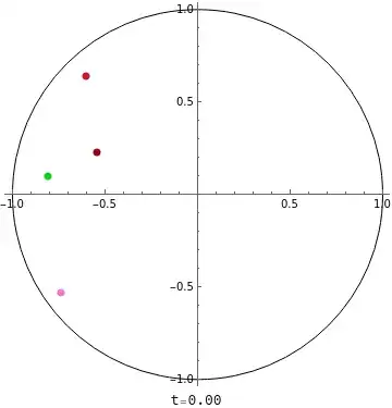
data = NBodySimulation[
    Association[
        "PairwisePotential" -> "Coulomb",
        "Region" -> Disk[],
        "ExternalForce" -> (Piecewise[{
            {-0.5 Normalize[#["Velocity"]], Norm[#["Velocity"]] > 10^-1},
            {0, Norm[#["Velocity"]] <= 10^-1}
        }] &)
    ],
    Association[
        "Mass" -> 1,
        "Position" -> #,
        "Velocity" -> {0, 0},
        "Charge" -> 10^-5
    ]& /@ initPos
, countTime];
colors = RandomColor[n];
Manipulate[
    Graphics[
        {Circle[], Red, PointSize[0.02], Riffle[colors, Point /@ data[All, "Position", time]]}
    , Axes -> True]
, {time, $MachineEpsilon, countTime, Appearance -> "Labeled"}]

Addendum. This is an explicit explanation as to why the Normalize part blows up in NDSolve. User @xzczd insists otherwise, further claiming that Normalize doesn't transform into anything, such as x/Abs[x]. While that's partially true, it's only when the input is already given as a number. When NDSolve computes a step, it first turns the terms containing variables/target function in the equation into their effective numerical form as much as possible, such as Normalize[{x'[t],y'[t]}] to {x'[t]/Norm[{x'[t],y'[t]}],y'[t]/Norm[{x'[t],y'[t]}]} and then to {x'[t]/Sqrt[Abs[x'[t]^2+y'[t]^2]],y'[t]/Sqrt[Abs[x'[t]^2+y'[t]^2]]}. One can easily check this:

Trace[NDSolve[{Normalize[{f[t], 0}] == {f'[t], 0}, f[0] == 1}, f, {t, 0, 1}]][[1, 1, 1]]
(* {Normalize[{f[t], 0}], {f[t]/Abs[f[t]], 0}} *)

Now, in the case of damping, if "Velocity" or numerical f'[t] gets small at some sufficiently large step (sufficient enough to kill off the precision) during NDSolve, then it's straightforward f'[t]/Abs[f'[t]] blows up:

q1 = 1`10;
q2 = 1`10 + 1/5*10^-9;
dq = q2 - q1;
Precision /@ {q1, q2, dq}
(* {10., 10., 0.} *)
dq/Norm[dq]
(* Error encountered; Indeterminate *)

One workaround is to define the function (damper) piecewise, for small Norm. This is precisely what I did above, which effectively solved the problem.

edited Feb 26 '22 at 09:58

answered Feb 25 '22 at 08:08

Shin Kim

1,271
3
9

The solution works, but the explanation isn't quite right, actually Normalize[{0, 0}] evaluates to {0, 0}. – xzczd Feb 25 '22 at 09:36
@xzczd Not quite. 0 is specially returning 0. Otherwise Normalize[x] is equivalent to x/Abs[x]. – Shin Kim Feb 25 '22 at 09:39
That's what I meant. There's no blow up. – xzczd Feb 25 '22 at 09:47
@xzczd Normalize[...] never jumps to 0 when ... is a floating number. You're suggesting that Normalize[{0,0}]={0,0} but this doesn't have much point because {0,0} has infinite precision, whereas NDSolve handles floating numbers. A better argument would have been suggesting Normalize[{0., 0.}]={0.,0.}, but when NBodySimulation gets a result having overshooting precision (i.e., higher than the working precision), it returns singularity or stiff system suspected or, in other words, blowing up. – Shin Kim Feb 25 '22 at 10:15
But you claimed that "This is because of your external force blowing up". The reason why ndsz warning pops up in this case isn't immediatly clear, but I'm pretty sure it's not caused by blowing up of external force. Also, observing the solution up to t==4.09 suggests the solution doesn't blow up, either. (ndsz warning doesn't necessarily mean there's a blow-up, see e.g. https://mathematica.stackexchange.com/a/219656/1871 , you can find more by searching ndsz in this site. ) – xzczd Feb 25 '22 at 10:26
@xzczd I'm sorry, but I don't see much reason to continue this conversation when you're not supporting your claim with reasons other than "it just doesn't blow up". I can't seem to find much useful info in the link you provided either. Try this: s=NDSolve[{q''[t] == -1/Abs[q'[t]], q[0] == 0, q'[0] == 0.1}, q, {t, 0, 1}] which is a simplified version, which, of course, also blows up (Plot[q[x] /. s, {x, 0.0045, 0.0050}, PlotRange -> All]). Mind you, Normalize[x] is equal to x/Abs[x] for floating x. – Shin Kim Feb 25 '22 at 10:45
As mentioned at beginning, the only thing I want to say is, your explanation is wrong. Normalize[x] never blow up, x/Abs[x] cannot be simplified to 1/Abs[x]. As long as x is a non-zero vector, Normalize always manages to normalize x. Try e.g. Normalize[{10^-100., 10^-100.}]. – xzczd Feb 25 '22 at 11:01
@xzczd Okay, I see where you're missing now. That argument is not quite relevant in NDSolve for couple of reasons. As I mentioned, NDSolve carries over every (floating) number with its working precision. When it handles Normalize[q'], it's doing q'/Norm[q']. If q' has piled up precision from many iterations of NDSolve at some step, then q'/Norm[q'] blows up because Norm[q'] becomes effectively 0. due to working precision having lower precision. This is why NDSolve returns ndsz. – Shin Kim Feb 25 '22 at 11:51
"When it handles Normalize[q'], it's doing q'/Norm[q']." Why do you think so? Normalize is never transformed to anything else, this can be easily proved by checking the NDSolve\StateData[…]object. Trysd = First@First@Flatten@Trace[NBodySimulation[……], _NDSolve`StateData]; sd["NumericalFunction"]["FunctionExpression"]Also, thendsz` warning can be circumvented by setting another ODE solver, see my answer. – xzczd Feb 25 '22 at 12:05
"When NDSolve computes a step, it first turns the terms containing variables/target function in the equation into their effective numerical form as much as possible, such as Normalize[{x'[t],y'[t]}]" But this doesn't happen in OP's case because NBodySimulation internally defines implicit vectors, just like in e.g. Trace[NDSolveValue[{Normalize[f[t]] == f'[t], f[0] == {1, 1}}, f, {t, 0, 1}]]. Once again, please check the NDSolve\StateData[…]` carefully. – xzczd Feb 26 '22 at 10:16
Another way to prove ndsz is not related to "blow up of Normalize" is to define Normalize as a black-box which will never be expanded for symbolic vectors: normalize[a : {_?NumericQ, _?NumericQ}] := Normalize[a] The ndsz warning still pops up at t=4.09 with normalize instead of Normalize in OP's code. – xzczd Feb 26 '22 at 10:22
@xzczd I don't think I deserve a negative vote from someone who's not willing to be a little more critical other than constantly insisting/giving vague arguments. Firstly, what StateData are you referring to? Also, what do you mean by implicit vectors? Lastly, of course it blows up again, as you effectively defined a tautological statement - try doing normalize[{q, q}] /. q -> 1, and piecewise define your normalize and see if it still works (it does). – Shin Kim Feb 26 '22 at 10:30
sd = First@First@ Flatten@Trace[ NBodySimulation[ Association["PairwisePotential" -> "Coulomb", "Region" -> Disk[], "ExternalForce" -> (Quantity[-0.5 Normalize[ QuantityMagnitude[#["Velocity"]]](*An extra damping*), "Newtons"] &)], <| "Mass" -> Quantity[1, "Kilograms"], "Position" -> Quantity[#, "Meters"], "Velocity" -> Quantity[{0, 0}, "Meters"/"Seconds"], "Charge" -> Quantity[10^-5, "Coulombs"]|> & /@ initPos, countTime], _NDSolve\StateData]; sd["NumericalFunction"]["FunctionExpression"]`

xzczd

Feb 26 '22 at 10:34

@xzczd I'm sorry, but your syntax doesn't seem to be correct - sd is empty and so it shows only errors. Edit: now it works. – Shin Kim Feb 26 '22 at 10:36

By implicit vector I mean something like f[t] in NDSolveValue[{Normalize[f[t]] == f'[t], f[0] == {1, 1}}, f, {t, 0, 1}], f[t] is not expressed as a explicit list {…} in the code, but it's undoubtedly a vector. 3. "try doing normalize[{q, q}] /. q -> 1…"So what? Can you make it expand to something involving Norm[{q, q}]?

– xzczd Feb 26 '22 at 10:39

How to make all the balls move until they stop by NBodySimulation

3 Answers3

Solution 1

Solution 2

Remark