How to predict the delay of a digital filter?

Question

I define a simple digital filter.

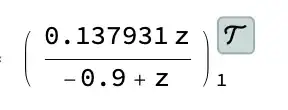
transferFunction = TransferFunctionModel[{{{0.13793103448275862*z}}, {{-0.9 + z}}}, z,SamplingPeriod -> 1]

Then I put samples of a sine wave in the filter.

input = Table[Sin[0.1 t], {t, 0, 250}];
filtered = RecurrenceFilter[transferFunction, input];
output = Transpose[{Range[1, Length@filtered], filtered}];

I found that after it reaches steady-state the filter output matches up very close with Sin[0.1*(t-8.101)]. How could we predict a 8.101 sample delay of that input using transferFunction above?

**** Correction *****

My code agrees with (delay = -7.10179) if make one change in computing input. The corrected code is:

input=Table[Sin[0.1 t],{t,1,250}];
filtered=RecurrenceFilter[transferFunction,input];
output=Transpose[{Range[1,Length@filtered],filtered}];
Plot[Sin[0.1(t-7.1)],{t,210,245},Epilog->{Point@output}]

andre314 · Accepted Answer · 2022-02-25T19:05:09.383

(* your code sligthly modified*)
transferFunction = 
 TransferFunctionModel[{{{0.13793103448275862*z}}, {{-0.9 + z}}}, z, 
  SamplingPeriod -> 1]
pulsation = .1;
input = Table[Sin[pulsation t], {t, 0, 250}];
filtered = RecurrenceFilter[transferFunction, input];
output = Transpose[{Range[1, Length@filtered], filtered}];

(* calculus of the exact delay *)
delay = transferFunction[Exp[pulsation I]] //
   RightComposition[
    #[[1, 1]] & 
    , ReIm 
    , ArcTan @@ #  &
    , (#  /pulsation &)
    ];

(* verification *)
ListLinePlot[{input, output, 
  MapIndexed[{First[#2] - delay, #1} &, input]},
 BaseStyle -> AbsoluteThickness[5], 
 PlotStyle -> {Black, Red, Directive[AbsoluteThickness[2], Green]},
 AspectRatio -> .2, ImageSize -> 900, 
 PlotLegends -> {"input", "output", "input delayed"}]

The exact delay is 7.1 seconds.

(However, I find the following much easier to understand.) tf=Part[transferFunction@Exp[pulsation I],1,1]; delay=ArcTan[Re@tf,Im@tf]/pulsation — Ted Ersek, Feb 25 '22 at 21:57
I just realize that "pulsation" is only a French word. In English it's "pulsatance" — andre314, Mar 02 '22 at 21:17

score 3 · Answer 2 · answered Feb 25 '22 at 15:35

Your frequency of interest turns out to be very close to the unity gain frequency. Assuming that this is no coincidence, work at that frequency.

samplingPeriodSeconds = 1;
transferFunction = TransferFunctionModel[{{{0.13793103448275862*z}}, {{-0.9 + z}}}, z, SamplingPeriod -> samplingPeriodSeconds]
phaseMargin = GainPhaseMargins[transferFunction][[2]]

unityGainFrequency = phaseMargin[[1, 1]]

0.100181

unityGainPhaseRadians = (Pi - phaseMargin[[1, 2]]);
unityGainSamplesPerCycle = 2*Pi*samplingPeriodSeconds / unityGainFrequency;
unityGainDelaySamples = unityGainSamplesPerCycle * unityGainPhaseRadians/(2*Pi)

7.0971

This suggests around 7.1 samples of delay. Perhaps you are miscounting one sample at the end. Plot for confirmation:

input = Table[Sin[unityGainFrequency*t], {t, 0, 250}];
filtered = RecurrenceFilter[transferFunction, input];
delayed = Table[Sin[unityGainFrequency ( t - unityGainDelaySamples)], {t, 0, 250}];
ListPlot[{input, filtered, delayed}, PlotRange -> {{0, 100}, Full},  PlotLegends -> {"input", "filtered", "delayed"}]

How to predict the delay of a digital filter?

2 Answers2

Linked