7

For finding inflection points for function
f[x_] := x^Sin[x]

I use f''[x]

Then Solve : Solve[f''[x] == 0, x]

But MMA is not capable calculating the 6 zero points symbolic. So it must be done numerical. What solve strategies are possible ?

Note : for a extra root solving method see also FindRoot

janhardo
  • 659
  • 3
  • 12
  • 3
    All computer algebra systems like Mathematica,Maple is not capable calculating the 6 zero points symbolic ,because in math there is no theory describing the solution to this topic. – Mariusz Iwaniuk Mar 02 '22 at 15:50

4 Answers4

8
Clear["Global`*"];

f[x_] := x^Sin[x]

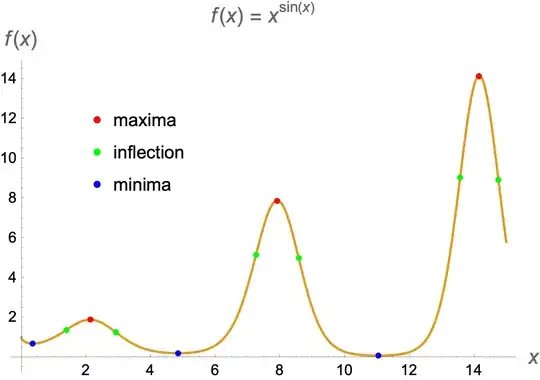
The local maxima occur at

argmax =
 NSolve[{f'[x] == 0, f''[x] < 0, 0 <= x <= 15}, x, Reals]

(* {{x -> 2.12762}, {x -> 7.91498}, {x -> 14.1638}} *)

The local minima occur at

argmin =
 NSolve[{f'[x] == 0, f''[x] > 0, 0 <= x <= 15}, x, Reals]

(* {{x -> 0.352215}, {x -> 4.84256}, {x -> 11.0333}} *)

The inflection points occur at

arginfl =
 NSolve[{f''[x] == 0, 0 <= x <= 15}, x, Reals]

(* {{x -> 1.39529}, {x -> 2.9161}, {x -> 7.25862}, {x -> 8.57615}, {x -> 13.5721}, {x -> 14.7568}} *)

Graphically,

Plot[f[x], {x, 0, 15},
 PlotStyle -> ColorData[97][2],
 Epilog -> {AbsolutePointSize[4],
   Red, Point[{x, f[x]} /. argmax],
   Blue, Point[{x, f[x]} /. argmin],
   Green, Point[{x, f[x]} /. arginfl]},
 AxesLabel -> (Style[#, 14] & /@ {x, HoldForm[f[x]]}),
 PlotLabel -> Style[StringForm["`` = ``",
    HoldForm[f[x]], f[x]], 14],
 PlotLegends -> Placed[
   PointLegend[{Red, Green, Blue},
    {"maxima", "inflection", "minima"}],
   {0.25, 0.7}]]

enter image description here

Bob Hanlon
  • 157,611
  • 7
  • 77
  • 198
  • Thanks, that's clear: all conditions for min, max function values are included in the NSolve command. – janhardo Mar 02 '22 at 14:59
5

A purely graphical approach using MeshFunctions + Mesh + RegionFunction:

plots = MapThread[
   Plot[f[x], {x, 0, 18}, 
     PlotRange -> All, Axes -> False, Frame -> True, ImageSize -> Large, 
     PlotStyle -> #, 
     MeshFunctions -> {Function[{x, y}, #2]}, Mesh -> {{0}}, 
     MeshStyle -> {Directive[AbsolutePointSize[10], #3]},
     RegionFunction -> Function[{x, y}, #4], 
     PlotLegends -> PointLegend[{Directive[AbsolutePointSize[8], #3]}, {#5}]] &, 
   {{Thick, None, None}, 
    {f''[x], f'[x], f'[x]}, 
    {Blue, Red, Green}, 
    {True, f''[x] < 0, f''[x] > 0}, 
    Style[#, 16] & /@ {"inflection", "max", "min"}}];

xticks = Flatten[Cases[Normal @ #, {Directive[___, c_?ColorQ], pts : {__Point}} :> Thread[Style[Round[pts[[All, 1, 1]], .001], c, 14, Bold, Opacity[1]]], All] & /@ plots];

Show[plots, FrameTicks -> {{Automatic, Automatic}, {{#[[1]], Rotate[#, 90 Degree]} & /@ xticks, Automatic}}]

enter image description here

GroupBy[xticks, #[[2]] /. 
   Thread[{ Blue, Red, Green} -> {"inflection", "max", "min"}] & ->  First,
  Sort]

enter image description here

See also: This answer by Silvia

kglr
  • 394,356
  • 18
  • 477
  • 896
5

An NDSolve solution, because I like NDSolve and it's just hanging around on my laptop. (Note: Function to be plotted must be smooth.)

calcPlot[x^Sin[x],
 {x, 0, 20},
 MeshStyle -> {PointSize@Medium},
 PlotLegends -> Placed[calcPlot["Legend"], {0.25, 0.75}]]

enter image description here

The solutions are cached:

calcPlot["CPs"]
(*
<|"Min" -> {{4.84255, 0.209274}, {0.352214, 0.697671}, {11.0333, 
    0.0907897}, {17.299, 0.0578358}}, 
 "Max" -> {{7.91498, 7.88459}, {2.12762, 1.89828}, {14.1638, 
    14.1505}, {20.4366, 20.4284}}, 
 "IP" -> {{8.57615, 5.01558}, {7.25862, 5.16106}, {2.9161, 
    1.27035}, {1.39529, 1.38816}, {13.5721, 9.048}, {14.7568, 
    8.94732}, {19.8785, 12.9545}, {20.9952, 12.8718}}|>
*)

Code dump:

Options through the Method option of ListLinePlot:

  • "CPs" (which solutions to collect & show, among {"Root", "Min", "Max", "IP"}).
  • "CPStyles" (colors for the points).
  • "NDSolveOptions" (options passed to NDSolve).

Also if PlotLegends contains calcPlot["Legend"], it will be replaced by a PointLegend[].

calcPlot // ClearAll;
calcPlot["CPs"] = <||>; (* last result cache *)
calcPlot[f_, {x_, a_, b_}, opts : OptionsPattern[ListLinePlot]] := 
 Module[{y, x0, meth, cps, styles, ndopts, legend},
  (*
  starting point with a 'random' offset:
  events are not detected on the first step 
  so we try to avoid symmetry
  *)
  x0 = (a (1 + Sqrt@$MachineEpsilon) + 
      b (1 - Sqrt@$MachineEpsilon))/2;
  (* Method options *)
  meth = OptionValue[Method];
  If[! OptionQ[meth], meth = {}];
  cps = Replace["CPs" /. meth,
    {"CPs" -> {"Min", "Max", "IP"},
     s_String :> {s},
     All -> {"Root", "Min", "Max", "IP"},
     Except[{___String}] :> {}}];
  styles = 
   Replace[
    "CPStyles" /. 
     meth, {"CPStyles" -> {"Root" -> Darker@Yellow, "Min" -> Magenta, 
       "Max" -> Purple, "CP" -> Red, "IP" -> Darker@Green, _ -> Black},
     s : {___} :> Append[s, _ -> Black],
     s_Rule :> {s, _ -> Black}
     }];
  ndopts = Replace["NDSolveOptions" /. meth, {"NDSolveOptions" -> {}}];
  legend = OptionValue[PlotLegends] /. Automatic -> calcPlot["Legend"];
  If[! FreeQ[legend, calcPlot["Legend"]],
   With[{leg = legend}, 
    legend := leg /. calcPlot["Legend"] :>
       PointLegend[
        Replace[Keys@calcPlot["CPs"], styles, 1],
        Keys@calcPlot["CPs"],
        Joined -> {False}] (* override ListLinePlot *)
    ]
   ];
  Reap[ (* calculate graph & critical points *)
    NDSolveValue[{
      y'''[x] == D[f, {x, 3}],
      y[x0] == f /. x -> x0,
      y'[x0] == D[f, x] /. x -> x0,
      y''[x0] == D[f, {x, 2}] /. x -> x0,
      WhenEvent[y[x] == 0, {Sow[{x, y[x]}, "Root"]}],
      WhenEvent[(x - x0) y'[x] > 0, {Sow[{x, y[x]}, {"CP", "Min"}]}],
      WhenEvent[(x - x0) y'[x] < 0, {Sow[{x, y[x]}, {"CP", "Max"}]}],
      WhenEvent[y''[x] == 0, {Sow[{x, y[x]}, "IP"]}]}, y,
     (* offset to avoid singularities at end points *)
     {x, 
      a + (b - a) $MachineEpsilon, b - (b - a) $MachineEpsilon},
     ndopts,
     MaxStepFraction -> 1/50, (* since we're plotting *)
     (* try not to skip an event near the start: *)
     StartingStepSize -> (b - a) Sqrt@$MachineEpsilon/10],
    cps,
    Rule] // (* process results: *)
   ListLinePlot[First@#,
     PlotLegends :> legend,
     opts,
     Epilog -> {
       Replace[
        OptionValue@MeshStyle, {Automatic -> {}, 
         o_List :> Directive @@ o}],
       calcPlot["CPs"] = Association@*Join @@ Last@#;
       KeyValueMap[
        {Replace[#1, styles],
          Point /@ #2} &,
        calcPlot["CPs"]]},
     PlotRange -> All] &
  ];
Michael E2
  • 235,386
  • 17
  • 334
  • 747
4

There are an infinite number of turning points. Restricting the range NSolve evaluates as desired:

NSolve[{f''[x] == 0, 0 < x < 20}, x]
(*{{x -> 1.39529}, {x -> 2.9161}, {x -> 7.25862}, {x -> 8.57615}, {x -> 13.5721}, {x -> 14.7568}, {x -> 19.8785}}*)
Ulrich Neumann
  • 53,729
  • 2
  • 23
  • 55
  • Which syntax variation is this for NSolve? i.e, {f''[x] == 0, 0 < x < 20}. In the docs, I see NSolve[expr,vars] and NSolve[expr,vars,Reals] for v12.2.0? – Syed Mar 02 '22 at 11:32
  • @Ulrich Neumann , thanks , when using Maple there are at least three solving commands to find, but in MMA its simple..there is only one..good – janhardo Mar 02 '22 at 11:33
  • @Syed NSolve allows constraints as first argument too – Ulrich Neumann Mar 02 '22 at 11:34
  • @Syed - The syntax given is "NSolve[expr, vars] attempts to find numerical approximations to the solutions of the system expr of equations or inequalities for the variables vars" (emphasis added). The constraints are the inequalities in the system. – Bob Hanlon Mar 02 '22 at 13:59
  • Ulrich Neumann and Bob Hanlon: Thanks to both of you for your clarifications. – Syed Mar 02 '22 at 14:05