How to solve the einstein field equation symbolically?

Question

How can I use Mathematica to solve the disturbed Einstein field equation? Is there any notebook that introduces this subject or package like diffgeo?

Answer 1

1. I would like to say that I have a preference of avoiding any packages, unless absolutely necessary. I prefer to have full control. This is not to say that this is the right way of doing things. Hence, this answer is not the unique approach to the problem.

2. To other (more experienced) members: I am certain that there are posts here that explain what I am about to do so if you could leave some links in the comment section, I will make sure to incorporate them in the main body. Many thanks in advance.

3. To the author of the OP: please consider upvoting the older answers that will come as suggestions. It is a very easy task and rewarding good and helpful answers is important of other users as well. Many thanks!

4. Based on Hartle's material.

Some background notes: in the OP there isn't an explicit metric, and hence I will be using the $\mathrm{AdS}_5$ spacetime in the Poincar`{e} parameterization, i.e

$$ \begin{equation} ds^2 = \frac{1}{u^2_0} \left(\eta_{\mu \nu} dx^{\mu} dx^{\nu} + du^2_0 \right) \end{equation} $$
with $\eta_{\mu \nu}$ in the (correct) mostly plus signature. I am using this particular one for convenience and because it is easy to check results against pen and paper computations.

Comment 1 What you need to understand is that you can input the metric tensor as a list of lists to correctly account for the number of indices and the dimensionality of the spacetime. Hopefully, this will be clear.

Comment 1.1 Please do keep in mind that the command MatrixForm is for display purposes ONLY.

Comment 2 Curvature tensors and scalars are essentially derivatives and contractions. In order to perform differentiation, Part is the command you want to look up in the docs. After declaring your coordinates it should look like this

D[list1[[s, j]], list2[[k]]]

with list1 the metric input and list2 the list of coordinates. In order to do contractions, you need to Sum over the index/indices that are contracted for the allowed values. Finally, for free indices we have Table.

Start the code

We declare our coordinates and the dimensionality of the spacetime under consideration

coord = {t, x1, x2, x3, u0};
dim = Length@coord;

Now, we proceed to define the metric components. metric are the components of the form $G_{AB}$ and its inverse are the indices up.

metric = 1/
   u0^2 {{-1, 0, 0, 0, 0}, {0, 1, 0, 0, 0}, {0, 0, 1, 0, 0}, {0, 0, 0,
      1, 0}, {0, 0, 0, 0, 1}};
inversemetric = Simplify[Inverse@metric];

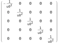
You can check how it looks like this

MatrixForm@metric

First easy manipulation -that appears in many physics applications

Sqrt[-Det@metric] // PowerExpand // FullSimplify

1/u0^5

---

Step 1 Coding the Christoffel symbols. Their mathematical definition is:

$$ \begin{equation} \Gamma^{i}_{kj} = \frac{1}{2}g^{is}\left(\partial_k g_{sj} + \partial_j g_{sk} - \partial_s g_{jk} \right) \end{equation} $$

The code for them

affine = FullSimplify[Table[(1/2)*Sum[(inversemetric[[i, s]])*
       (D[metric[[s, j]], coord[[k]] ] +
         D[metric[[s, k]], coord[[j]] ] - 
         D[metric[[j, k]], coord[[s]] ]), {s, 1, dim}],
    {i, 1, dim}, {j, 1, dim}, {k, 1, dim}]];

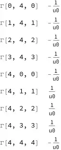
This is enough, and if you call affine you can see all the components of the Christoffel. However, there's a neat way of displaying them. We are showing all the non-trivial and independent components of the Christoffel; recall they have a symmetry:

listaffine := 
 Table[If[UnsameQ[affine[[i, j, k]], 
    0], {ToString[Γ[i - 1, j - 1, k - 1]], 
    affine[[i, j, k]]}] , {i, 1, dim}, {j, 1, dim}, {k, 1, j}]
TableForm[Partition[DeleteCases[Flatten[listaffine], Null], 2], 
 TableSpacing -> {2, 2}]

Note: Γ[x1,x2,x3] is $\Gamma^{x1}_{x2,x3}$.

Now this should be enough as a helpful demonstration for you to code the other curvature invariants. Again, remember they follow the same philosophy, derivatives and contractions.

Anyway, I will give some extra stuff below:

---

Step 2 Coding the coordinate expression of the Riemann tensor

riemann = 
  Simplify[Table[
    D[affine[[i, j, l]], coord[[k]] ] - 
     D[affine[[i, j, k]], coord[[l]] ] + 
     Sum[affine[[s, j, l]] affine[[i, k, s]] - 
       affine[[s, j, k]] affine[[i, l, s]],
      {s, 1, dim}], {i, 1, dim}, {j, 1, dim}, {k, 1, dim}, {l, 1, 
     dim}]];
listriemann := 
 Table[If[UnsameQ[riemann[[i, j, k, l]], 
    0], {ToString[R[i - 1, j - 1, k - 1, l - 1]], 
    riemann[[i, j, k, l]]}] , {i, 1, dim}, {j, 1, dim}, {k, 1, 
   dim}, {l, 1, k - 1}]
TableForm[Partition[DeleteCases[Flatten[listriemann], Null], 2], 
 TableSpacing -> {2, 2}]

---

Step 3 Coding the Ricci tensor

ricci = FullSimplify[
   Table[Sum[riemann[[i, j, i, l]], {i, 1, dim}], {j, 1, dim}, {l, 1, 
     dim}]];
listricci := 
 Table[If[UnsameQ[ricci[[j, l]], 0], {ToString[R[j - 1, l - 1]], 
    ricci[[j, l]]}] , {j, 1, dim}, {l, 1, j}]
TableForm[Partition[DeleteCases[Flatten[listricci], Null], 2], 
 TableSpacing -> {2, 2}]

---

Step 4 Coding the Ricci scalar

scalar = FullSimplify[
  Sum[inversemetric[[i, j]] ricci[[i, j]], {i, 1, dim}, {j, 1, dim}]]

-20

---

Step 5 Coding the Kretschmann scalar

We need to contract the Riemann tensor. riemann1 is the tensor with all indices down and riemann2 with all indices up.

riemann1 = 
  Simplify[Table[
    Sum[metric[[\[Mu], \[Mu]1]]*
      riemann[[\[Mu]1, \[Nu], \[Rho], \[Sigma]]], {\[Mu]1, 1, 
      dim}], {\[Mu], 1, dim}, {\[Nu], 1, dim}, {\[Rho], 1, 
     dim}, {\[Sigma], 1, dim}]];
listriemann1 := 
  Table[If[UnsameQ[riemann1[[\[Mu], \[Nu], \[Rho], \[Sigma]]], 
     0], {ToString[R1[\[Mu], \[Nu], \[Rho], \[Sigma]]], 
     riemann1[[\[Mu], \[Nu], \[Rho], \[Sigma]]]}], {\[Mu], 1, 
    dim}, {\[Nu], 1, dim}, {\[Rho], 1, dim}, {\[Sigma], 
    1, \[Rho] - 1}];
TableForm[Partition[DeleteCases[Flatten[listriemann1], Null], 2], 
  TableSpacing -> {2, 2}];
riemann2 = 
  Simplify[Table[
    Sum[Sum[Sum[
       inversemetric[[\[Nu]1, \[Nu]]]*
        inversemetric[[\[Rho]1, \[Rho]]]*
        inversemetric[[\[Sigma]1, \[Sigma]]]*
        riemann[[\[Mu], \[Nu]1, \[Rho]1, \[Sigma]1]], {\[Nu]1, 1, 
        dim}], {\[Rho]1, 1, dim}], {\[Sigma]1, 1, dim}], {\[Mu], 1, 
     dim}, {\[Nu], 1, dim}, {\[Rho], 1, dim}, {\[Sigma], 1, dim}]];
listriemann2 := 
  Table[If[UnsameQ[riemann2[[\[Mu], \[Nu], \[Rho], \[Sigma]]], 
     0], {ToString[R2[\[Mu], \[Nu], \[Rho], \[Sigma]]], 
     riemann2[[\[Mu], \[Nu], \[Rho], \[Sigma]]]}], {\[Mu], 1, 
    dim}, {\[Nu], 1, dim}, {\[Rho], 1, dim}, {\[Sigma], 
    1, \[Rho] - 1}];
TableForm[Partition[DeleteCases[Flatten[listriemann2], Null], 2], 
  TableSpacing -> {2, 2}];
KretschmannScalar = 
 Simplify[Sum[
   riemann1[[a, b, c, d]]*riemann2[[a, b, c, d]], {a, 1, dim}, {b, 1, 
    dim}, {c, 1, dim}, {d, 1, dim}]]

40

---

Step 6 Coding the Einstein tensor

einstein = Simplify[ricci - (1/2) scalar*metric];
listeinstein := 
 Table[If[UnsameQ[einstein[[j, l]], 0], {ToString[G[j, l]], 
    einstein[[j, l]]}] , {j, 1, dim}, {l, 1, j}]
TableForm[Partition[DeleteCases[Flatten[listeinstein], Null], 2], 
 TableSpacing -> {2, 2}]

---

Step 7 Please persuade yourself that the above statements are correct for the AdS spacetime.

---

Step 8 Since you now have the code for all this, it should be easy to code the matrix components of the vielbein basis - the orthonormal basis- and from that to get the the spin-connection components. This is a good exercise. You can try to do it and if you can't just leave a comment.

---

Step 9 Understanding what a metric perturbation is: a metric perturbation around an ambient spacetime, is just shifts in the tensor by something, i.e

$$ g_{ab} + \epsilon h_{ab} $$

where $\epsilon$ is a small parameter. Can you see how to go about it now?