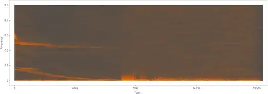
I did the ShortTimeFourier(stf) Transformation of the following signal.
And got the results as shown in this Spectrogram.
Then I wanted to find the peak frequency of this each turn using PeakDetect as:
Qpeak = Table[PeakDetect[GaussianFilter[Abs[stf[[b]]["Data"][[turn]]], \[Sigma]], \[Sigma]/ 2, 0, qthreshold], {b, numpeaks}];
And plot it using MatrixPlot as below for 80 numpeaks.

I want to convert this bin # into the frequency. There are 1024 bins as I selected ShortTimeFourier partition length as 1024 (https://reference.wolfram.com/language/ref/ShortTimeFourier.html.en). To my knowledge, 1024 bins represent frequencies from -0.5 to 0.5. I don't know if the first half (up to 512 bins) shows -0.5 to 0 and second half (513-1024 bins) shows 0 to 0.5 frequency range or other way around.
Could you please help me with this? I appreciate any help you can provide.
CODE
xtrain = Import[dir <> "xtrain.dat"];
ListPlot[Evaluate@{#[[1]] & /@ xtrain, #[[10]] & /@
    xtrain,  #[[40]] & /@ xtrain,  #[[70]] & /@
    xtrain,  #[[10000]] & /@ xtrain, #[[18000]] & /@ xtrain},
 Joined -> True, PlotRange -> All, PlotTheme -> "Scientific",
 FrameLabel -> {"Bunch #", "[Proportional] x position"} ,
 PlotLabel -> "Bunch train behaviour for different turns",

 PlotLegends -> {1, 10, 40, 70, 10000, 18000}, ImageSize -> 500]
(I have 80 bunches in each turn and have 20000 turns)
ListPlot[Evaluate@{# & /@ xtrain[[1]]},  Joined -> True,
 PlotRange -> All, PlotTheme -> "Scientific",
 FrameLabel -> {"Turn #", "\[Proportional] x position"} ,
 ImageSize -> 500]

(For a single bunch this is how x position vs time (turn) plot looks
like which I want to do Fourier Transformation)
ShortTimeFourier
npointFFT = 1024;
nskip = 10;
ncols = Round[Length[xtrain[[1]]]/nskip];
dcol =  ncols/npointFFT // N ;
stf = Table[
   ShortTimeFourier[# & /@ xtrain[[i]], npointFFT, nskip], {i,
    Length[xtrain]}];
oldxticks = {0, 2500, 5000, 7500, 10000};
xticks = {#, Round[# dcol]} & /@ oldxticks;
(Spectrogram of stf for bunch 1)
gf1 = Spectrogram[stf[[1]],
  FrameLabel -> {"Turn #", "Betatron tune"},
  PlotLabel -> "Bunch 1 spectrogram",
  FrameTicks -> {{Automatic, None}, {xticks, None}},
  PlotTheme -> "Marketing", ImageSize -> 1000]

Find the peak frequency for each turn in each bunch
qthreshold = 0.15;
Qtrain1[t_] :=
  Module[{Qpeak, turn, \[Sigma]},  (*for the gaussian fit*)
   turn = Round[t];
   If[turn < 50, \[Sigma] = 32, \[Sigma] = 16];
   If[turn < 600, qthreshold = 0.15];
   If[turn >= 600, qthreshold = 0.15];
   Qpeak =
    Table[ PeakDetect[
      GaussianFilter[
       Abs[stf[[b]]["Data"][[turn]]], \[Sigma]], \[Sigma]/2, 0,
      qthreshold], {b, numpeaks}];
   (*MatrixPlot[Reverse[Transpose[Qpeak]], FrameLabel-> {"Q",
   "Bunch #"},FrameTicks->{{Automatic, Automatic}, {Automatic,None}}]*)
MatrixPlot[Qpeak, FrameLabel -> {"Q", "Bunch #"},
    FrameTicks -> {{yticks, Automatic}, {Automatic, None}}]
   ];
Qtrain1[1] (for turn 1)

Plot the amplitude vs frequncy plot
turn = 1; (*for turn 1, bunch 1*)
If[turn < 50, \[Sigma] = 32, \[Sigma] = 16];
If[turn < 600, qthreshold = 0.15];
If[turn >= 600, qthreshold = 0.15];
Qpeak = Table[
   PeakDetect[
    GaussianFilter[Abs[stf[[b]]["Data"][[turn]]], \[Sigma]], \[Sigma]/
     2, 0, qthreshold], {b, numpeaks}];
b = 1;
gg2 = ListPlot[{Abs[stf[[b]]["Data"][[turn]]],
   GaussianFilter[
    Abs[stf[[b]]["Data"][[turn]][[startQ ;; stopQ]]], [Sigma]],
   Qpeak[[b]] GaussianFilter[
     Abs[stf[[b]]["Data"][[turn]][[startQ ;; stopQ]]], [Sigma]]},
  Joined -> True, PlotRange -> All, PlotStyle -> {Green, Dashed, Red},
   Joined -> {True, True, False}, Filling -> {3 -> 0},
  FillingStyle -> Opacity[1], PlotTheme -> {"Classic", "Frame"},
  PlotLabel ->
   "Turn = " <> ToString[(turn - 1) nskip + 1] <> " bunch = " <>
    ToString[b], FrameLabel -> {"Bin #", "Amplitude"},
  Epilog -> {Line[{{0, qthreshold}, {1024, qthreshold}}]}]
 `
`
Data file:
https://drive.google.com/file/d/1mZ5TIphAwG3QkwywFH96cq4B598RVTd3/view?usp=sharing