0

I know the values for a function v[x,y] on an irregular grid of (x,y) points. Call the table storing all these points xyvtriples. Because of the irregular grid, the Mathematica function Interpolation only works as

interpolatedvfunc = Interpolation[xyvtriples, InterpolationOrder -> 1];

But what I really need are the partial derivatives of interpolatedfunc with respect to each argument, and for those partials to be continuous, which won't happen due to the edges produced by InterpolatioOrder -> 1.

Is there any way around this? I can make a very fine grid of (x,y) points to (I hope) counter any problems with forcing a spline like interpolation if I can somehow force this to happen.

Thanks.

cphelan
  • 23
  • 2
  • If NDSolve can do it, you can, too: (E.g. usol = NDSolve[{-Laplacian[u[x, y], {x, y}] == 1, DirichletCondition[u[x, y] == 0, True]}, u, {x, y} \[Element] Disk[]]; Plot3D[Evaluate[D[u[x, y], x] /. First[usol]], {x, y} \[Element] Disk[]]. But I don't understand your setup/workflow and feel it's not worth trying something out I don't really need and don't know if it will help. Please give a minimal working example (in code) for us to copy/paste and play with. – Michael E2 Apr 16 '22 at 15:06
  • 1
    You say that you can make a very fine grid of $(x,y)$ points; what, then, is stopping you from making this fine grid so regular that Interpolation will accept it at higher order? – Roman Apr 16 '22 at 15:45
  • This may be an XY problem. If you tell us how you calculate the values of your $v(x,y)$, then maybe somebody can suggest a direct way of calculating the partial derivatives instead of taking a detour over interpolation and numerical differentiation. – Roman Apr 16 '22 at 15:46
  • 1

2 Answers2

1

You could use the first interpolation to create data on a grid. Then you can interpolate this new data with the default InterpolationOrder->3. Here is an example:

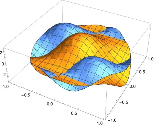
f1 = Interpolation[dat, InterpolationOrder -> 1] Plot3D[f1[x, y], {x, 0, 2 Pi}, {y, 0, 2 Pi}]

enter image description here

Now we can create new data and interpolate it:

dat2 = Table[{x, y, f1[x, y]}, {x, 0, 2 Pi}, {y, 0, 2 Pi}] f2 = Interpolation[dat]; Plot3D[f2[x, y], {x, 0, 2 Pi}, {y, 0, 2 Pi}]

enter image description here

Finally you can get the partial derivatives.

Daniel Huber
  • 51,463
  • 1
  • 23
  • 57
1

I can make a very fine grid of (x,y) points to (I hope)...

I hope to have guessed the OP's setup/workflow...and that this quote indicates that the data/function to be interpolated can be generated for any set of points.

In which case, we can use a quadratic ElementMesh[] to get a higher-order interpolation.

Needs@"NDSolve`FEM`";
emesh = ToElementMesh[Disk[]];
data = Function[{x, y}, Sin[3 x] Cos[2 y]^2] @@@ 
   emesh["Coordinates"]; (* need data pt for each of these coords *)
ifn = ElementMeshInterpolation[{emesh}, data];
Plot3D[Evaluate[D[ifn[x, y], {{x, y}}]], {x, y} \[Element] emesh]

Being order 2, ifn is not of class $C^2$:

Plot3D[Evaluate[D[ifn[x, y], {x, 2}]], {x, y} \[Element] emesh, 
 PlotPoints -> 100, NormalsFunction -> None, Mesh -> None]
Michael E2
  • 235,386
  • 17
  • 334
  • 747