2

I'm new with Mathematica and I have a problem with that, It would be great if you could help me with that. I try to draw a maximum slope of a plot in the same diagram using resource function tangent line, but it seams that it doesn't work for complex function.

ClearAll;
$Assumptions = 
  n ∈ Reals && z ∈ Reals && znew ∈ Reals;

z = Sqrt[2 epsilon] E^(n); ztwotransitions = Sqrt[2 epsilontwotransitions] E^(n); znew = Sqrt[2 epsilonnew] E^(n); epsilon = aminus1^2/( 18 MPL^2 H0^4) (1 - (aminus1 - aplus)/ aminus1 E^(-3 (n - n0new)))^2; epsilontwotransitions = aminus1^2/( 18 MPL^2 H0^4) (1 - (aminus1 - aplus)/aminus1 E^(-3 (n - n0)))^2; epsilonnew = astar^2/(18 MPL^2 H0^4) (1 - (astar - aminus2)/ astar E^(-3 (n - n1)))^2; modefristsr = 1/Sqrt[2 k] (1 - I/(k τ)) E^(-I k τ); modefristsrprime = D[modefristsr, τ]; modensr = c1/Sqrt[2 k] (1 - I/(k τ)) E^(-I k τ) + c2/Sqrt[2 k] (1 + I/(k τ)) E^(I k τ); modensrprime = D[modensr, τ]; modesecondsr = d1/Sqrt[2 k] (1 - I/(k τ)) E^(-I k τ) + d2/Sqrt[2 k] (1 + I/(k τ)) E^(I k τ); modesecondsrprime = D[modesecondsr, τ]; modefristsrn = Evaluate[modefristsr /. τ -> -1/H0 E^(-n)]; modefristsrprimen = Evaluate[modefristsrprime /. τ -> -1/H0 E^(-n)]; modensrn = Evaluate[modensr /. τ -> -1/H0 E^(-n)]; modensrprimen = Evaluate[modensrprime /. τ -> -1/H0 E^(-n)]; modesecondsrn = Evaluate[modesecondsr /. τ -> -1/H0 E^(-n)]; modesecondsrprimen = Evaluate[modesecondsrprime /. τ -> -1/H0 E^(-n)]; modefristsrn0new = Evaluate[modefristsrn /. n -> n0new]; modefristsrprimen0new = Evaluate[modefristsrprimen /. n -> n0new]; modensrn0new = Evaluate[modensrn /. n -> n0new]; modensrprimen0new = Evaluate[modensrprimen /. n -> n0new]; eqns = {modefristsrn0new - modensrn0new == 0 && modensrprimen0new - modefristsrprimen0new == f0 modensrn0new}; c1c2 = Solve[eqns, {c1, c2}]; solevedmodensrn = modensrn /. c1c2; modefristsrn0 = Evaluate[modefristsrn /. n -> n0]; modefristsrprimen0 = Evaluate[modefristsrprimen /. n -> n0]; modensrn0 = Evaluate[modensrn /. n -> n0]; modensrprimen0 = Evaluate[modensrprimen /. n -> n0]; eqnswithf2 = {modefristsrn0 - modensrn0 == 0 && modensrprimen0 - modefristsrprimen0 == f2 modensrn0}; c11c21 = Solve[eqnswithf2, {c1, c2}]; solvedfirstslowroll = modefristsrn /. c1c2; solevedmodensrnnew = modensrn /. c11c21; solevedmodensrn1 = Evaluate[solevedmodensrnnew /. n -> n1]; solvedmodensrprimen = modensrprimen /. c11c21; solvedmodensrprimen1 = Evaluate[solvedmodensrprimen /. n -> n1]; modesecondsrn1 = Evaluate[modesecondsrn /. n -> n1]; modesecondsrprimen1 = Evaluate[modesecondsrprimen /. n -> n1]; d1d2 = Solve[ solevedmodensrn1 - modesecondsrn1 == 0 && modesecondsrprimen1 - solvedmodensrprimen1 == f1 solevedmodensrn1, {d1, d2}]; solevedmodesecondsrn = modesecondsrn /. d1d2; powerwithc1c2 = k^3/(2 π^2) (z^(-2)) Abs[solevedmodensrn]^2; powerwithd1d2 = k^3/(2 π^2) (znew^(-2)) Abs[solevedmodesecondsrn]^2; f0 = 3 k0new ( aminus1 - aplus)/aplus; f1 = 3 k1 (astar - aminus2)/aminus2; f2 = 3 k0 (aminus - aplus)/aplus; MPL = 1; a = E^(n); k1 = a1 H0; a0 = E^(n0); a0new = E^(n0new); a1 = E^(n1); τ1 = 0.1; H0 = 8.8 10^(-7); σ = 0.01; astar = 7 10^(-16) MPL^3; aminus = 7.26 10^(-15) MPL^3; aplus = 3.35 10^(-14) MPL^3; deltaa = aminus1 - aplus; n0 = 10; n1 = 15; n0new = 10; k0 = a0 H0; k0new = a0new H0; aminus1 = 7 10^(-16); aminus2 = 7.26 10^(-15); LogLogPlot[ Evaluate[{powerwithc1c2 , powerwithd1d2} /. {k -> k0 kstar, n -> 200}], {kstar, 10^(-1), 1000} , AxesLabel -> {"!(*FractionBox[(k), (k0)])", "Power_Spectrum"}, PlotLegends -> {"one_transition", "Two_transitions"}]


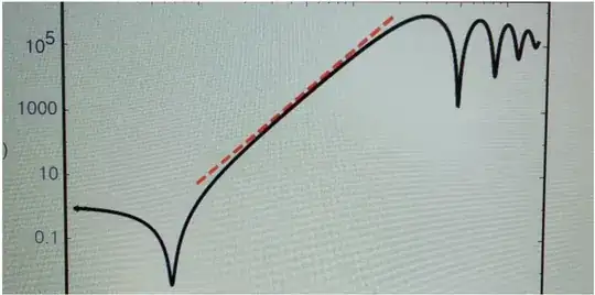
Edited post: This is what should how result should look like:
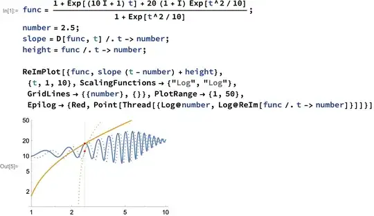
march
  • 23,399
  • 2
  • 44
  • 100
  • Do you mean complex as in complex numbers $z=x+iy$? Or complicated? – Michael E2 May 03 '22 at 14:17
  • I mean complex function as a function with imaginary part @Michael E2 – Alireza Madad May 03 '22 at 14:22
  • Then the tangent "line" to $w=f(z)$ is a complex line $w=\alpha z+\beta$, that is in terms of real coordinates, a two-dimensional plane in the four-dimensional space $(w,z)\in{\Bbb C}^2$, no? The only tools we have are ComplexPlot3D and ComplexPlot - not sure about log-log space. But something like this, maybe: func = (var^2 + 1)/(var^2 - 1); number = 1 + I; slope = D[func, var] /. var -> number; height = func /. var -> number; ComplexPlot3D[#, {var, -2 - I, 3 + 4 I}] & /@ {func, slope (var - number) + height} // Show – Michael E2 May 03 '22 at 14:40
  • Thanks a lot for your response but I want to show the tangent line in the diagram so complexplot does not help. I need to indicate the slope of the function in a specific point. @Michael E2 – Alireza Madad May 03 '22 at 14:46
  • I see 2 lines, I expect 2 tangent functions, isn't it? – yarchik May 03 '22 at 14:47
  • Just define the real and imaginary parts of the function, and treat them separately. – yarchik May 03 '22 at 14:48
  • What is your specific point? – yarchik May 03 '22 at 14:48
  • yes. there are two functions and I need to show slope for the both @yarchik – Alireza Madad May 03 '22 at 14:49
  • my specific point is k=k0 @yarchik – Alireza Madad May 03 '22 at 14:55
  • Just define the real and imaginary parts of the function, and treat them separately. it is very hard and complicated to do this @yarchik – Alireza Madad May 03 '22 at 14:57
  • I edited post and added a picture of how result should be look like @Michael E2 – Alireza Madad May 03 '22 at 15:23
  • I edited post and added a picture of how result should be look like @yarchik – Alireza Madad May 03 '22 at 15:23
  • Perhaps something like this: func = Exp[(10 I - 1) t]; number = 1/2; slope = D[func, t] /. t -> number; height = func /. t -> number; ReImPlot[{func, slope (t - number) + height}, {t, 0, 1}(*,ScalingFunctions->{"Log","Log"}*)] -- if you choose log-log space/scale, lines do not appear as lines (unless the y intercept is 0, in which case they all appear as having slope 1). You might like to have it drawn straight as in your image, but that's a misrepresentation. It can be done however, though it's tricky. – Michael E2 May 03 '22 at 16:05
  • Here's a related Q&A about tangents and LogPlot but about real-valued functions instead of complex-valued ones: https://mathematica.stackexchange.com/questions/57437/how-can-i-add-a-tangent-arrow-at-a-certain-point-of-a-curve-in-a-logplot – Michael E2 May 03 '22 at 17:06

1 Answers1

2

Here's an example. Linear functions do not have straight graphs under log-log scaling unless they pass through $(0,0)$, in which case their slopes appear as $m=1$ in loglog space. Note that extra graphics added by hand (such as the red points) have to be scaled by hand.

func = (1 + Exp[(10 I + 1) t] + 20 (1 + I) Exp[t^2/10])/(1 + Exp[t^2/10]);
number = 2.5;
slope = D[func, t] /. t -> number;
height = func /. t -> number;

ReImPlot[{func, slope (t - number) + height}, {t, 1, 10}, ScalingFunctions -> {"Log", "Log"}, GridLines -> {{number}, {}}, PlotRange -> {1, 50}, Epilog -> {Red, Point[Thread[{Log@number, Log@ReIm[func /. t -> number]}]]}]

Here's a way to draw the lines incorrectly but straight:

ReImPlot[func, {t, 1, 10}, ScalingFunctions -> {"Log", "Log"},
 GridLines -> {{number}, {}}, PlotRange -> {1, 50},
 Epilog -> {
   Red,
   Point[Thread[{Log@number, Log@ReIm[func /. t -> number]}]],
   ColorData[97][2],
   Riffle[
    {Dashing[{}], Dotted},
    InfiniteLine /@ Transpose@{
       Thread[{Log@t, Log@ReIm[func]} /. t -> number],
       Thread[{Log@t, Log@ReIm[func]} /. 
         t -> number (1 + Sqrt@$MachineEpsilon)]
       }
    ]
   }
 ]

I used a numerical approximation to the apparent slope in scaled loglog space (by taking the line through two nearly adjacent points), because it was easier and good enough for graphing.

Michael E2
  • 235,386
  • 17
  • 334
  • 747
  • func = {(9 E^(-2 n) H0^4 k^3 MPL^2 Abs[( E^((I E^-n k)/ H0) (1 + (I E^(2 n0new) f0 H0^2)/(2 k^3) + (I f0)/(2 k)) (1 + ( I E^n H0)/k))/(Sqrt[2] Sqrt[k]) - ( I E^(-((I E^-n k)/H0) + (2 I E^-n0new k)/H0) f0 (1 - (I E^n H0)/k) (I E^n0new H0 + k)^2)/( 2 Sqrt[2] k^(7/2))]^2)/( 2 aminus1^2 (1 - ((aminus1 - aplus) E^(-3 (n - n0new)))/ aminus1)^2 \[Pi]^2)} – Alireza Madad May 03 '22 at 18:38
  • number = 1; slope = D[func, k] /. k -> number; height = func /. k -> number; ReImPlot[{func, slope (k - number) + height}, {k, 1, 100}, ScalingFunctions -> {"Log", "Log"}, GridLines -> {{number}, {}}, PlotRange -> {1, 100}, Epilog -> {Red, Point[Thread[{Log@number, Log@ReIm[func /. k -> number]}]]}] – Alireza Madad May 03 '22 at 18:39
  • Coordinate {0, {Log[ 558016.9319389397 Re[ 2.718281828459045^((-2) $CellContextn) (1 + 46.85714285714286 2.718281828459045^((-3) (-10 + \ $CellContextn)))^(-2) Abs[ Complex[-0.0007803515115195993, 0.02012192791307727] 2.718281828459045^(Complex[0., 103.18165855110193` should be a pair of numbers, or a Scaled or Offset form . – Alireza Madad May 03 '22 at 18:40
  • Abs is not differentiable. – Michael E2 May 03 '22 at 18:41
  • Thanks a lot for your answer, I write your code and it did not work for my function and it gave the massage above, I don't know what I missed. I wrote the function I'm using.@ Michael E2 – Alireza Madad May 03 '22 at 18:42
  • I ticked your answer, thanks for your time, but any suggestion what should I do with Abs? – Alireza Madad May 03 '22 at 18:45
  • @AlirezaMadad So I think this gives the derivative: number = 1; slope = D[ComplexExpand@func, n] /. n -> number; height = func /. n -> number; ReImPlot[{func, slope (n - number) + height}, {n, 1, 100}, ScalingFunctions -> {"Log", "Log"}, GridLines -> {{number}, {}}, Epilog -> {Red, Point[Thread[{Log@number, Log@ReIm[height]}]] /. {_, _DirectedInfinity} -> Nothing}] -- BUT: There's a lot of numerical noise, which probably messes things up. PLUS: The slope is negative which makes the tangent have negative values that cannot be plotted on a log scale.... – Michael E2 May 03 '22 at 18:51
  • ...You needed to change a few things: Instead of k -> number, it should have been n -> number (right?). The PlotRange worked for my example, but not yours. The height is a real number, so its imaginary part is zero, and you can't take the log of it. That's what the {_, _DirectedInfinity} -> Nothing is for: to get rid of Log[0], which is infinity. – Michael E2 May 03 '22 at 18:54
  • it's working now, I'm quiet happy :) but still have problem, number should equal to k0 but it doesn't show the line, I don't know what range I should use. k0=8.8*10^(3) – Alireza Madad May 03 '22 at 20:31
  • This is my code: ReImPlot[Evaluate[{func, slope (k - number) + height} /. {k -> k0 kstar, n -> 100}], {kstar, 10^(-1), 100}, ScalingFunctions -> {"Log", "Log"}, GridLines -> {{number}, {}}, Epilog -> {Red, Point[Thread[{Log@number, Log@ReIm[height]}]] ColorData[97][2], Riffle[{Dashing[{}], Dotted}, InfiniteLine /@ Transpose@{Thread[{Log@k, Log@ReIm[func]} /. k -> number], Thread[{Log@k, Log@ReIm[func]} /. k -> number (1 + Sqrt@MachinEpsilon)]}] /. {_, _DirectedInfinity} -> Nothing}] – Alireza Madad May 03 '22 at 20:33