Three nonlinearly coupled PDEs

Question

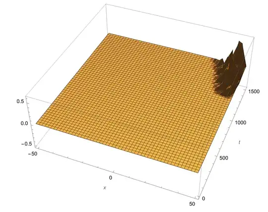
I am new to Mathematica and I need it to solve a system of three nonlinearly coupled PDEs.

$\frac{n_1}{c_0} \frac{\partial E_1}{\partial t}+\frac{\partial E_1}{\partial x} = i\frac{\omega_1}{2n_1 c_0} {\chi}^{(2)} g(x)E_2 E_3 e^{-i\Delta k x} $

$\frac{n_2}{c_0} \frac{\partial E_2}{\partial t}+\frac{\partial E_2}{\partial x} = i\frac{\omega_2}{2n_2 c_0} {\chi}^{(2)} g(x)E_1 E_3^{*} e^{i\Delta k x} $

$\frac{n_3}{c_0} \frac{\partial E_3}{\partial t}-\frac{\partial E_3}{\partial x} = i\frac{\omega_3}{2n_3 c_0} {\chi}^{(2)} g(x)E_1 E_2^{*} e^{i\Delta k x} $

These equations represent the nonlinear three wave-mixing under the slowly varying envelope approximation, in the situation of difference- frequency-generation. The Pump wave ($E_1$) has a Gaussian shape, while the other two waves are orders of magnitude smaller background fields made out of randomly-phased harmonic fields ($E_2$ & $E_3$). Additionally, one of the waves ($E_3$) counter-propagates relative to the other two.

My efforts to solve this with NDSolve were proven unsuccessful, as even when I de-couple the equations (by setting $g(x)=0$) or assume phase matching $\Delta k=0$, I get bad results. When StepSize is large I get some unwanted/unphysical ripples mostly for the counter propagating wave. $\E_3$" /> When I decrease the StepSize, the ripples start to show in the second background field ($E_2$), while the results for the counter-propagating wave gets completely wrong together with NDSolve::eerr warning. $E_3$" /> One of things I notice is that I get different results when changing the amplitude of the waves, although when de-coupled the solutions should only scale.

Although I tried to tweak several of the NDSolver options and configurations I couldn’t make it work. This is even before I turn on the coupling and/or experiments with different parameters. I included my code (also share my NOTEBOOK) and it would be amazing if someone could help me out. Thanks.

(* Parameters *)
c0 = 0.2998; (* speed of light in [um/fs] *)
n1 = 2.3;
n2 = 2.1;
n3 = 2;
L = 100; (* [um] *)
lam0P = 1.064; (* [um] *)
lam0I = 2.0; (* [um] *)
lam0S = 1/(lam0P^-1 - lam0I^-1); (* [um] *)
chi2 = 8*10^-6 ; (* [um/V] *)
ax = 1.0; (* chi2 modulation length [um] *)
tauP = 150; (* pulse duration [fs] *)
T = L*n1/c0 + 5*tauP; (*max time for evaluation*)
A = 100; (* [um^2] *)
E01 = 10000; (* Pump Peak E [V/um]*)
E0 = 0.0845; (* background fields amplitude [V*um]*)
nx = 4; (*number of points in a domain*)
(* Other variables )
om1 = c0/n12Pi/lam0P
om2 = c0/n22Pi/lam0S
om3 = c0/n32Pi/lam0I
E02 = (n2Llam0SA)^(-1/2) * E0; (background modes amplitudes)
E03 = (n3Llam0IA)^(-1/2)  E0;
omc2 = Pic0/(Ln2); (background modes frequencies)
omc3 = Pic0/(Ln3);
Pulse[t_] := Exp[-(t - 3*tauP)^2/tauP^2];
g[x_] = 0; (* SquareWave[x/ax-ax/nx*0.25]; )  ( [Chi]2 modulation )
Phibg = IRandomReal[{-Pi, Pi}, 8]; (random phases)
(* Equations, Boundaries and Initial Conditions )
(coupled PDEs)
eq1 = D[E1[x, t], t] == -c0 /n1(D[E1[x, t], x] + Iom1/(n1c0)chi2g[x]E2[x, t]E3[x, t]);
eq2 = D[E2[x, t], t] == -c0/n2(D[E2[x, t], x] + Iom2/(n2c0)chi2g[x]E1[x, t]Conjugate[E3[x, t]]);
eq3 = D[E3[x, t], t] == c0/n3(D[E3[x, t], x] + Iom3/(n3c0)chi2g[x]E1[x, t]Conjugate[E2[x, t]]);
(* initial conditions )
ic1 := E1[x, 0] == E01  Pulse[0];
ic2 := E2[x, 0] == E02(Exp[Iomc2n2/c0x + Phibg[[1]]] + Exp[I2omc2n2/c0x + Phibg[[2]]] + Exp[I3omc2n2/c0x + Phibg[[3]]] + Exp[I4omc2n2/c0x + Phibg[[4]]]);
ic3 := E3[x, 0] == E03(Exp[-Iomc3n3/c0x + Phibg[[5]]] + Exp[-I2omc3n3/c0x + Phibg[[6]]] + Exp[-I3omc3n3/c0x + Phibg[[7]]] + Exp[-I4omc3n3/c0x + Phibg[[8]]]);
(boundary conditions)
bc1 := E1[-L/2, t] == E01 * Pulse[t];
bc2 := E2[-L/2, t] == E02(Exp[-Iomc2t -Iomc2n2/c0L/2 + Phibg[[1]]] + Exp[-I2omc2t - Iomc2n2/c0L + Phibg[[2]]] +Exp[-I3omc2t - I3omc2n2/c0L/2 + Phibg[[3]]] + Exp[-I4omc2t - I2omc2n2/c0L + Phibg[[4]]]);
bc3 := E3[L/2, t] == E03(Exp[-Iomc3t - Iomc3n3/c0L/2 + Phibg[[5]]] + Exp[-I2omc3t - Iomc3n3/c0L + Phibg[[6]]] + Exp[-I3omc3t - I3omc3n3/c0L/2 + Phibg[[7]]] + Exp[-I4omc3t - I2omc3n3/c0L + Phibg[[8]]]);
sol = NDSolve[{eq1, eq2, eq3, ic1, ic2, ic3, bc1, bc2, bc3}, {E1,E2,E3}, {x, -L/2, L/2}, {t, 0, T}, Method -> {"MethodOfLines", "SpatialDiscretization" -> {"TensorProductGrid", "MinStepSize" -> ax/(2nx), "MaxStepSize" -> ax/(2nx)}}]