A strategy to create good initial guess for Lorentzian model fit

Question

I was preparing an answer for a question that got deleted, so I will post this anyhow.

Given a set of data with a hump

data = Import["https://pastebin.com/raw/DMhcUZAQ","CSV"]

that one may want to fit to a Lorentzian model

model = a/((t - b)^2 + d) + c;

How to create a good initial guess for all the fit parameters?

That should include estimates for:

Centre
Width
Peak value
Baseline

or equivalent parameters.

Thank you for drafting this! I was also working on an alternative approach to the same question, and I was frustrated when it was deleted. — MarcoB, Jul 12 '22 at 16:10
+1 on both question and answer. Just curious: Is this simulated data? I ask because dividing all of the responses by 0.004 results in integers (which suggests either simulations or that the response consists of counts which might then suggest Poisson regression). — JimB, Jul 12 '22 at 16:32
@JimB Not sure. The data comes from this deleted question. It was part of a series of similar questions from the same user, who at some point mentioned that it was related to high resolution laser spectroscopy. Passing familiarity with the field suggests that the raw measurements were indeed integer counts. — MarcoB, Jul 12 '22 at 17:05

rhermans · Answer 1 · 2022-07-12T15:54:30.953

The initial guess

We load the data

data = Import["https://pastebin.com/raw/DMhcUZAQ","CSV"]

The guess components

centre = Total[Times@@@data]/Total[data[[All,2]]]; (* Centroid *)
{base,peak}= MinMax[data[[All,2]]];  (* Vertical range *)
{xmin,xmax}= MinMax[data[[All,1]]];  (* Horizontal range *)
width = (Power[data[[All,1]] - centre,2].data[[All,2]])/Total[data[[All,2]]] (* Width *)

The model

model = a/((t - b)^2 + d) + c;

the complete guess

fitguess = {{a, peak*width}, {b, centre}, {c, base}, {d, width}}

Let's see if it's any close

Show[
    ListPlot[
        data
        ,PlotStyle->Blue
        ,PlotTheme->"Scientific"
    ],
    Plot[
        Evaluate[model/.Rule@@@fitguess]
        ,{t,xmin,xmax}
        ,PlotStyle->Red
    ]
]

not too bad for an initial guess.

The actual fit

fit = NonlinearModelFit[data
    , model
    , fitguess
    , t
];
Show[
    dataplot,
    Plot[
        Evaluate[fit[x]]
        ,{x,xmin,xmax}
    ]
]

score 6 · Answer 2 · answered Jul 12 '22 at 16:07

I would recommend using a model of the Lorentzian curve that more explicitly highlights the meaning of the parameters:

newmodel = area/Pi width/((t - peak)^2 + width^2);

In the model above, the position of the peak is indicated by peak, the curve's width parameter by width, and the area under the curve is given directly by area, as one can confirm below:

assumptions = {width > 0, peak ∈ Reals, area > 0};
(* Area under the curve )
Integrate[newmodel, {t, -Infinity, Infinity}, Assumptions -> assumptions]
( Out: area *)
(* Value at max )
valueAtMax = Simplify[MaxValue[newmodel, t], Assumptions -> assumptions]
( Out: area/(π width) *)
(* full width at half maximum = 2width )
Solve[newmodel == valueAtMax/2, t]
(* Out: {{t -> peak - width}, {t -> peak + width}} *)

With this model, fitting is easier as well:

data = Import["https://pastebin.com/raw/DMhcUZAQ", "CSV"];
result = NonlinearModelFit[data, newmodel, {width, peak, area}, t];
result["BestFitParameters"]
(* Out: {width -> 198.68, peak -> 4959.41, area -> 215.959} *)
Show[
  ListPlot[data], 
  Plot[result[t], {t, 4370, 5600}, PlotStyle -> Red, PlotRange -> Full]
]

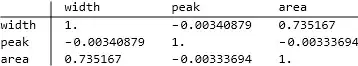
The only caveat is the fact that the area and width parameters are somewhat correlated:

TableForm[
  result["CorrelationMatrix"],
  TableHeadings -> {{"width", "peak", "area"}, {"width", "peak", "area"}}
]

With this, one would be in a better position to optimize the starting values of the parameters thanks to a more immediate grasp of their physical meaning.

A strategy to create good initial guess for Lorentzian model fit

2 Answers2

The initial guess

The actual fit

Linked