I have a Matlab-style code that uses Fourier transform efficiently. Here is the function which defines a differentiation matrix D, where N denotes the modes number and kk is the wavenumber.
function [A,B,D,x]=func(N)
dxx=2*pi/N;x=dxx*((1:N)');
kk=[-N/2+1:N/2]';
C=diag(1i*kk);
A=exp(1i*x*kk');
B=exp(-1i*kk*x')/N;
D=A*(C*B);
In the main program, the differentiation matrix D can be used easily as an operator. For example, consider a function y(x). It uses a couple of lines to calculate the 1st- to 3rd-order derivatives.
N=64;
[A,B,D,x]=func(N);
D1=real(D);
D2=real(D^2);
D3=real(D^3);
Dy=D1y;
D2y=D2y;
D3y=D3*y;
I want to convert it exactly equivalently into Mathematica. I note that Mathematica provides the functions FourierTransform and FourierCoefficient, however, I found it has various parameter values for several different conventions, which is confusing. Can anyone please help to convert it as Mathematica code, and if you could give an example, it will be very helpful!
Update
Thanks for the help of @J. M.'s persistent exhaustion and @user293787, I can calculate the 1st- and 2nd-order derivatives, but when using the code to calculate the 3rd-order derivative, the error is too large to be acceptable. I also tried use more modes with $n=256$, but the computational time became longer and the result became worse. Can you help to improve it? Thank you very much!
f3d[n_] := Module[{kk = Range[-n/2 + 1, n/2], x = 2*\[Pi]*Range[n]/n},
Exp[I*KroneckerProduct[x, kk]].DiagonalMatrix[(I kk)^3].(Exp[-I*KroneckerProduct[kk, x]]/n)]
n = 128; (n = 256;)
(an exmaple)
f[x_] := Sin[x] Cos[3 x] + Sin[4 x];
vals = Table[N[f[x], 20], {x, -[Pi], [Pi], 2 [Pi]/(n - 1)}];
dddf = D[f[x], {x, 3}];
dddvals = Re[N[f3d[n], 20]].vals;
dddvalsTrue = Table[N[dddf, 20], {x, -[Pi], [Pi], 2 [Pi]/(n - 1)}];
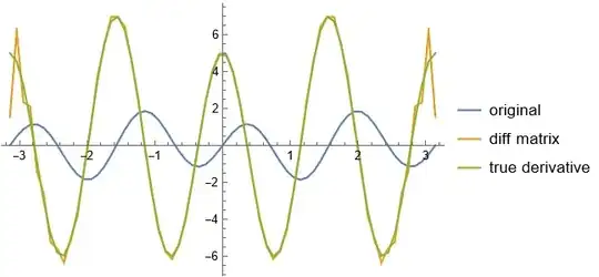
thirdDplot = ListLinePlot[{vals, dddvals, dddvalsTrue}, DataRange -> {-[Pi], [Pi]}, PlotLegends -> {"original func", "diff matrix", "Exact derivative"}]

{x,-\[Pi],\[Pi]-2 \[Pi]/n,2 \[Pi]/n}in your tables, or something like that. But maybe this is getting out of hand here, I think @J.M. answered your original question. – user293787 Jul 23 '22 at 09:54Tablein my update should be modified. Could you explain a little? – user95273 Jul 23 '22 at 12:15x-value is $-\pi$ and the second is $+\pi$, which is the same point in a $2\pi$-periodic setting. Also, the stepsize must match the stepsize that you use inExp[I*KroneckerProduct[x, kk]]which is $2\pi/n$. – user293787 Jul 23 '22 at 12:18NDSolve`FiniteDifferenceDerivative?: https://mathematica.stackexchange.com/q/182295/1871 – xzczd Jul 27 '22 at 05:32Pseudospectralwe should use a mesh with uniform nodes. However, in that link the author of that post used a non-uniform mesh. Could please write a short answer to show how to use your functionfunc = NDSolveFiniteDifferenceDerivative[1, x, DifferenceOrder -> "Pseudospectral"]` to calculate the 3rd-order derivative of the example in the update of my post? Thank you again! – user95273 Jul 27 '22 at 14:32grid = N@Range[-Pi, Pi, 2 Pi/25]; val = NDSolve`FiniteDifferenceDerivative[3, grid, f@grid, DifferenceOrder -> "Pseudospectral", PeriodicInterpolation -> True]; ListPlot[{grid, val}\[Transpose]]~Show~Plot[f'''[x], {x, -Pi, Pi}]"when usingPseudospectralwe should use a mesh with uniform nodes" Yes, but only ifPeriodicInterpolation -> True. Otherwise we need the Chebyshev-Gauss-Lobatto grid. Please read the document more carefully. – xzczd Jul 27 '22 at 14:45