If I understood it correctly, you can try this:
pdf[x_, y_] := (a0 + a1 + a2)*((a1*a2)/a0)*Exp[-a1 x - a2 y]*(1 - Exp[-a0 Min[x, y]])
and then, assigning the value of 1 to a0, a1 and a2, you can plot it:
Plot3D[Evaluate@pdf[x, y] /. {a0 -> 1, a1 -> 1, a2 -> 1},
  {x, 0, 4}, {y, 0, 6}, ColorFunction -> "Rainbow",
  PlotRange -> All, Mesh -> Full, Exclusions -> None]
Result:

EDITED
If you want to "simulate" from the continuous probability distribution, you might want to use Manipulate[] to see what happens when you change parameters a0, a1 and a2:
Manipulate[
  Plot3D[Evaluate@pdf[x, y] /. {a0 -> v0, a1 -> v1, a2 -> v2}, {x, 0, 4}, {y, 0, 4},
  ColorFunction -> "Rainbow", PlotRange -> All,
  Mesh -> Full, Exclusions -> None],
  {{v0, 1, "a0"}, .001, 1, .001},
  {{v1, 1, "a1"}, .001, 1, .001},
  {{v2, 1, "a2"}, .001, 1, .001}]
Result:

EDITED
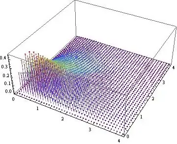
The discrete case:
DiscretePlot3D[Evaluate@pdf[x, y] /. {a0 -> 1, a1 -> 1, a2 -> 1},
  {x, 0, 4, .1}, {y, 0, 4, .1}, ColorFunction -> "Rainbow", PlotRange -> All]
Result:
EDITED
You could also plot the ContourPlot[] of your distribution:
ContourPlot[pdf[x, y] /. {a0 -> 1, a1 -> 1, a2 -> 1},
  {x, 0, 4}, {y, 0, 4}, ColorFunction -> "Rainbow",
  PlotRange -> All, Exclusions -> None]
Result:

RandomVariate[]andProbabilityDistribution[]. – J. M.'s missing motivation Jun 18 '13 at 06:26