Numerical solution for overdetermined, albeit well posed 1st order PDE system

Question

I'm trying to solve for $\theta(u,v)$ defined by the system

\begin{align} \partial_v h+h\:\partial_u\theta=0\\ \partial_u h-h\:\partial_v\theta=0 \end{align}

being $\log h(u,v)$ a given harmonic function. The condition $(\partial^2_{u}+\partial^2_v)\log h=0$ guarantees that $\partial^2_{uv}\theta=\partial^2_{vu}\theta$, so the system is know to be well defined and its solution exists up to a constant $\theta(u_0,v_0)$. For simple enough $h$, DSolve returns the analytic solution, however when moving to NDSolve I get the alert of overdetermined system and no answer.

 h[u_, v_] := u^2 + v^2
 NDSolveValue[{D[h[u, v], v] + h[u, v]*D[θ[u, v], u] == 0, 
               D[h[u, v], u] - h[u, v]*D[θ[u, v], v] == 0, 
               θ[0, 0] == 0}, θ, {u, 0.1, 1}, {v, 0.1, 1}]

Answer 1

OK, let me provide a solution based finite difference method (FDM). The idea is simple (and it's not the first time I use it, see this post for another example): the system is overdetermined in form, so we use LeastSquare to solve it.

I'll use pdetoae for generation of difference equation system.

h[u_, v_] := u^2 + v^2
sys = {D[h[u, v], v] + h[u, v] D[θ[u, v], u] == 0, 
       D[h[u, v], u] - h[u, v] D[θ[u, v], v] == 0, 
       θ[0, 0] == 0};
points@u = points@v = 50; 
domain@u = domain@v = {0, 1}; 
(grid@# = Array[# &, points@#, domain@#]) & /@ {u, v};
difforder = 2;
(* Definition of pdetoae isn't included in this post,
   please find it in the link above. )
ptoafunc = pdetoae[θ[u, v], grid /@ {u, v}, difforder];
aesys = {ptoafunc@Most@sys, Last@sys} // Flatten // DeleteCases[True];
vars = Outer[θ, grid@u, grid@v] // Flatten;
{barray, marray} = CoefficientArrays[aesys, vars];
sollst = LeastSquares[marray, -N@barray]; // AbsoluteTiming
( {0.712605, Null} *)
solmat = ArrayReshape[sollst, points /@ {u, v}];
sol = ListInterpolation[solmat, grid /@ {u, v}];
Plot3D[sol[u, v], {u, #, #2}, {v, #3, #4}] & @@ Flatten[domain /@ {u, v}]

Let's compare it with the exact solution -2 ArcTan[u/v] provided by Alex in the comment below:

With[{eps = 10^-3}, 
 Manipulate[
  Plot[{sol[u, v], const - 2 ArcTan[u/v]}, {u, eps, 1}, PlotRange -> All, 
   PlotStyle -> {Automatic, Dashed}], {v, eps, 1}, {{const, 1.5}, 1, 2}]]

Remark

1. The ratio points@u/points@v will influence the solution by a constant. (This isn't a problem, of course. ) This is probably because function value θ[0, 0] only exists as a limit in certain direction.

2. You can set the b.c. at other points of the domain e.g. θ[49/50, 49/50] == 0 for points@u = points@v = 51.

Answer 2

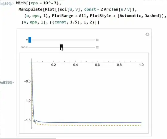
As an alternative method we can use the Euler wavelets collocation method described in our paper and on my page. We add one equation $\theta_1=\int{\theta_u du},\theta_2=\int{\theta_v dv}, \theta_1=\theta_2$. With this method we can solve the problem on the grid $16\times 16$ with absolute error of $4\times 10^{-3}$. First, we define exact solution

h[u_, v_] := 
 u^2 + v^2; sys = {Derivative[0, 1][h][u, v] + 
    h[u, v] D[\[Theta][u, v], u] == 0, 
  Derivative[1, 0][h][u, v] - h[u, v] D[\[Theta][u, v], v] == 
   0, \[Theta][0, 0] == 0};
DSolveValue[{D[h[u, v], v] + h[u, v]*D[\[Theta][u, v], u] == 0, 
  D[h[u, v], u] - h[u, v]*D[\[Theta][u, v], v] == 0, \[Theta][0, 0] ==
    Pi/2}, \[Theta], {u, v}]
(Out[]= Function[{u, v}, 1/2 ([Pi] - 4 ArcTan[u/v])])

With this exact solution we can test our numerical solution. Second, we compute numerical solution

UE[m_, t_] := EulerE[m, t]
psi[k_, n_, m_, t_] := 
 Piecewise[{{2^(k/2) UE[m, 2^k t - 2 n + 1], (n - 1)/2^(k - 1) <= t < 
     n/2^(k - 1)}, {0, True}}]
PsiE[k_, M_, t_] := 
 Flatten[Table[psi[k, n, m, t], {n, 1, 2^(k - 1)}, {m, 0, M - 1}]]
k0 = 3; M0 = 4; With[{k = k0, M = M0}, 
 nn = Length[Flatten[Table[1, {n, 1, 2^(k - 1)}, {m, 0, M - 1}]]]];
dx = 1/(nn);  xl = Table[ l*dx, {l, 0, nn}]; ucol = 
 vcol = Table[(xl[[l - 1]] + xl[[l]])/2, {l, 2, nn + 1}]; Psijk = 
 With[{k = k0, M = M0}, PsiE[k, M, t1]]; Int1 = 
 With[{k = k0, M = M0}, Integrate[PsiE[k, M, t1], t1]];
Psi[y_] := Psijk /. t1 -> y; int1[y_] := Int1 /. t1 -> y;
M = nn;
U1 = Array[a, {M, M}]; U2 = Array[b, {M, M}]; G1 = 
 Array[g1, {M}]; G2 = Array[g2, {M}];
tet1[u_, v_] := int1[u] . U1 . Psi[v] + G1 . Psi[v]; 
tet2[u_, v_] := Psi[u] . U2 . int1[v] + G2 . Psi[u];
tetv[u_, v_] := Psi[u] . U2 . Psi[v];
tetu[u_, v_] := Psi[u] . U1 . Psi[v];
eq = Join[
   Flatten[Table[
     Derivative[0, 1][h][ucol[[i]], vcol[[j]]] + 
      h[ucol[[i]], vcol[[j]]] tetu[ucol[[i]], vcol[[j]]], {i, M}, {j, 
      M}]], Flatten[
    Table[Derivative[1, 0][h][ucol[[i]], vcol[[j]]] - 
      h[ucol[[i]], vcol[[j]]] tetv[ucol[[i]], vcol[[j]]], {i, M}, {j, 
      M}]], Flatten[
    Table[tet1[ucol[[i]], vcol[[j]]] - tet2[ucol[[i]], vcol[[j]]], {i,
       M}, {j, M}]], {tet1[0, 0], tet2[0, 0]}];
var = Join[Flatten[U1], Flatten[U2], G1, G2];
{vec, mat} = CoefficientArrays[eq, var];
sol = LeastSquares[mat // N, -vec];
rul = Table[var[[i]] -> sol[[i]], {i, Length[var]}];

Visualization of numerical and exact solution, and error for $\theta_1, \theta_2$

{Plot3D[Evaluate[tet1[u, v] /. rul], {u, .1, 1}, {v, .1, 1}, 
  ColorFunction -> Hue, Exclusions -> None], 
 Plot3D[-2 ArcTan[u/v] + Pi/2, {u, .1, 1}, {v, .1, 1}, 
  ColorFunction -> Hue], 
 Plot3D[Abs[-2 ArcTan[u/v] + Pi/2 - 
    Evaluate[tet1[u, v] /. rul]], {u, .1, 1}, {v, .1, 1}, 
  ColorFunction -> Hue, Exclusions -> None, PlotRange -> All], 
 Plot3D[Abs[-2 ArcTan[u/v] + Pi/2 - 
    Evaluate[tet2[u, v] /. rul]], {u, .1, 1}, {v, .1, 1}, 
  ColorFunction -> Hue, Exclusions -> None, PlotRange -> All]}

Answer 3

Since it is an overdetermined system this means that one equation is enough to solve it. So you can choose first one or second one:

h[u_,v_]:=u^2+v^2
f1=NDSolveValue[{D[h[u,v],v]+h[u,v]*D[\[Theta][u,v],u]==0,\[Theta][0,v]==0},\[Theta],{u,0.1,1},{v,0.1,1}];
f2=NDSolveValue[{D[h[u,v],u]-h[u,v]*D[\[Theta][u,v],v]==0,\[Theta][u,0]==0},\[Theta],{u,0.1,1},{v,0.1,1}];
Plot3D[f1[u,v]+\[Pi]/2,{u,0.1,1},{v,0.1,1}]
Plot3D[f2[u,v]-\[Pi]/2,{u,0.1,1},{v,0.1,1}]
Plot3D[Function[{u,v},1/2 (\[Pi]-4 ArcTan[u/v])][u,v],{u,0.1,1},{v,0.1,1}]
{f1[u,v]+\[Pi]/2,f2[u,v]-\[Pi]/2,Function[{u,v},1/2 (\[Pi]-4 ArcTan[u/v])][u,v]}/.{u->0.2,v->0.3}
(* {0.394725, 0.394815, 0.394791} *)

Results f1 and f2 differ from exact solution by constants +π/2 and -π/2. If you subtract these constants you get the same result.