Here's a way to use linear programming to get reasonably simple solutions. As an example, I'll do the Greek flag.
The flag is defined as a 18×27 matrix:
M = {{1, 1, 1, 1, 0, 0, 1, 1, 1, 1, 1, 1, 1, 1, 1, 1, 1, 1, 1, 1, 1, 1, 1, 1, 1, 1, 1},
     {1, 1, 1, 1, 0, 0, 1, 1, 1, 1, 1, 1, 1, 1, 1, 1, 1, 1, 1, 1, 1, 1, 1, 1, 1, 1, 1},
     {1, 1, 1, 1, 0, 0, 1, 1, 1, 1, 0, 0, 0, 0, 0, 0, 0, 0, 0, 0, 0, 0, 0, 0, 0, 0, 0},
     {1, 1, 1, 1, 0, 0, 1, 1, 1, 1, 0, 0, 0, 0, 0, 0, 0, 0, 0, 0, 0, 0, 0, 0, 0, 0, 0},
     {0, 0, 0, 0, 0, 0, 0, 0, 0, 0, 1, 1, 1, 1, 1, 1, 1, 1, 1, 1, 1, 1, 1, 1, 1, 1, 1},
     {0, 0, 0, 0, 0, 0, 0, 0, 0, 0, 1, 1, 1, 1, 1, 1, 1, 1, 1, 1, 1, 1, 1, 1, 1, 1, 1},
     {1, 1, 1, 1, 0, 0, 1, 1, 1, 1, 0, 0, 0, 0, 0, 0, 0, 0, 0, 0, 0, 0, 0, 0, 0, 0, 0},
     {1, 1, 1, 1, 0, 0, 1, 1, 1, 1, 0, 0, 0, 0, 0, 0, 0, 0, 0, 0, 0, 0, 0, 0, 0, 0, 0},
     {1, 1, 1, 1, 0, 0, 1, 1, 1, 1, 1, 1, 1, 1, 1, 1, 1, 1, 1, 1, 1, 1, 1, 1, 1, 1, 1},
     {1, 1, 1, 1, 0, 0, 1, 1, 1, 1, 1, 1, 1, 1, 1, 1, 1, 1, 1, 1, 1, 1, 1, 1, 1, 1, 1},
     {0, 0, 0, 0, 0, 0, 0, 0, 0, 0, 0, 0, 0, 0, 0, 0, 0, 0, 0, 0, 0, 0, 0, 0, 0, 0, 0},
     {0, 0, 0, 0, 0, 0, 0, 0, 0, 0, 0, 0, 0, 0, 0, 0, 0, 0, 0, 0, 0, 0, 0, 0, 0, 0, 0},
     {1, 1, 1, 1, 1, 1, 1, 1, 1, 1, 1, 1, 1, 1, 1, 1, 1, 1, 1, 1, 1, 1, 1, 1, 1, 1, 1},
     {1, 1, 1, 1, 1, 1, 1, 1, 1, 1, 1, 1, 1, 1, 1, 1, 1, 1, 1, 1, 1, 1, 1, 1, 1, 1, 1},
     {0, 0, 0, 0, 0, 0, 0, 0, 0, 0, 0, 0, 0, 0, 0, 0, 0, 0, 0, 0, 0, 0, 0, 0, 0, 0, 0},
     {0, 0, 0, 0, 0, 0, 0, 0, 0, 0, 0, 0, 0, 0, 0, 0, 0, 0, 0, 0, 0, 0, 0, 0, 0, 0, 0},
     {1, 1, 1, 1, 1, 1, 1, 1, 1, 1, 1, 1, 1, 1, 1, 1, 1, 1, 1, 1, 1, 1, 1, 1, 1, 1, 1},
     {1, 1, 1, 1, 1, 1, 1, 1, 1, 1, 1, 1, 1, 1, 1, 1, 1, 1, 1, 1, 1, 1, 1, 1, 1, 1, 1}};
ArrayPlot[M, ColorRules -> {0 -> White, 1 -> RGBColor["#004C98"]}, PlotRangePadding -> None]

We have many duplicate rows and columns in this flag, so let's restrict problem-solving to unique rows/columns, giving a reduced 5×3 flag to be expressed in terms of outer products:
M1 = M // Transpose // DeleteDuplicates // Transpose // DeleteDuplicates
(*    {{1, 0, 1}, {1, 0, 0}, {0, 0, 1}, {0, 0, 0}, {1, 1, 1}}    *)
{py, px} = Dimensions[M1]
(*    {5, 3}    *)
Let's make a list of all possible Kronecker products of a binary 5-list with a binary 3-list. The flag will be expressed as a linear combination of such Kronecker products. Each Kronecker product can appear with a positive or negative sign.
This is different from the OP's solution that uses contributions $\{-1,0,1\}$ and therefore finds a simpler solution. However, the present method can be extended to do this as well, I think.
p = Tuples[{{-1, 1}, Rest[Tuples[{0, 1}, py]], Rest[Tuples[{0, 1}, px]]}];
q = SparseArray[Flatten[#[[1]]*KroneckerProduct[#[[2]],#[[3]]]] & /@ p];
Find the linear combination of Kronecker products (in q) that (i) has the fewest contributing terms, (ii) has every term's prefactor restricted to $[0,1]$, and (iii) sums to express the reduced flag M1: the parameters given to LinearOptimization are
- the linear objective to be minimized: the sum of all term prefactors
- the linear inequality constraints: every prefactor must be in $[0,1]$
- the linear equality constraints: the terms must add up to
M1.
Expressed in matrix form,
s = LinearOptimization[
      ConstantArray[1, Length[q]],
      {Join[IdentityMatrix[Length[q], SparseArray], -IdentityMatrix[Length[q], SparseArray]],
       Join[ConstantArray[0, Length[q]], ConstantArray[1, Length[q]]]},
      {Transpose[q], -Flatten[M1]}]
(*    {0, 0, 0, 0, 0, 0, 0, 0, 0, 0, 0, 0, 0, 0, 0, 0, 0, 0, 0, 0, 0, 0, 0, 0, 0, 0,
       0, 0, 0, 0, 0, 0, 0, 0, 0, 0, 0, 0, 0, 0, 0, 0, 0, 0, 0, 0, 0, 0, 0, 0, 0, 0,
       0, 0, 0, 0, 0, 0, 0, 0, 0, 0, 0, 0, 0, 0, 0, 0, 0, 0, 0, 0, 0, 0, 0, 0, 0, 0,
       0, 0, 0, 0, 0, 0, 0, 0, 0, 0, 0, 0, 0, 0, 0, 0, 0, 0, 0, 0, 0, 0, 0, 0, 0, 0,
       0, 0, 0, 0, 0, 0, 0, 0, 0, 0, 0, 0, 0, 0, 0, 0, 0, 0, 0, 0, 0, 0, 0, 0, 0, 0,
       0, 0, 0, 0, 0, 0, 0, 0, 0, 0, 0, 0, 0, 0, 0, 0, 0, 0, 0, 0, 0, 0, 0, 0, 0, 0,
       0, 0, 0, 0, 0, 0, 0, 0, 0, 0, 0, 0, 0, 0, 0, 0, 0, 0, 0, 0, 0, 0, 0, 0, 0, 0,
       0, 0, 0, 0, 0, 0, 0, 0, 1/3, 0, 0, 0, 0, 0, 0, 0, 0, 0, 0, 0, 0, 0, 0, 0, 0,
       0, 0, 0, 0, 0, 0, 0, 0, 0, 0, 0, 0, 0, 0, 0, 0, 0, 0, 0, 0, 0, 0, 0, 0, 0, 0,
       0, 0, 0, 0, 0, 0, 0, 0, 0, 0, 0, 0, 0, 0, 1/3, 0, 0, 0, 0, 0, 0, 0, 0, 0, 0,
       0, 0, 0, 0, 0, 0, 0, 0, 0, 0, 0, 0, 0, 0, 0, 0, 0, 0, 0, 0, 1/3, 0, 0, 0, 0,
       0, 0, 0, 0, 0, 0, 0, 0, 0, 0, 0, 0, 0, 0, 0, 0, 0, 0, 0, 0, 0, 0, 0, 0, 0, 0,
       0, 0, 0, 0, 0, 0, 0, 0, 0, 0, 0, 0, 0, 0, 0, 0, 0, 0, 0, 0, 0, 0, 0, 0, 0, 0,
       1/3, 0, 0, 0, 0, 0, 0, 0, 0, 0, 0, 0, 0, 0, 0, 1/3, 0, 0, 0, 0, 0, 0, 1/3, 0,
       0, 0, 0, 0, 0, 0, 0, 0, 0, 0, 0, 0, 0, 0, 0, 0, 0, 0, 0, 0, 0, 0, 1/3, 0, 0,
       0, 0, 0, 0, 1/3, 0, 0, 0, 0, 0, 0, 0, 0, 0, 0, 0, 0, 0, 0, 0, 0, 0, 0, 0, 0,
       0, 0, 0, 0, 0, 0, 0, 0, 0, 0, 0, 0, 0, 0, 0, 0, 0, 0, 0, 0, 0, 0, 0, 0, 0}    *)
Note that for larger problems, this optimization will be done numerically using, for example, an interior-point method.
The resulting combination is quite sparse, containing only 8 terms:
f = s . ((#[[1]] kp[#[[2]], #[[3]]]) & /@ p)
(*    1/3 kp[{0, 0, 1, 0, 1}, {0, 1, 1}] +
      1/3 kp[{0, 1, 0, 0, 1}, {1, 1, 0}] +
      1/3 kp[{1, 0, 0, 0, 1}, {1, 1, 1}] +
      1/3 kp[{1, 0, 1, 0, 0}, {0, 0, 1}] +
      1/3 kp[{1, 0, 1, 0, 1}, {0, 0, 1}] +
      1/3 kp[{1, 1, 0, 0, 0}, {1, 0, 0}] +
      1/3 kp[{1, 1, 0, 0, 1}, {1, 0, 0}] -
      1/3 kp[{1, 1, 1, 0, 0}, {0, 1, 0}]      *)
where kp is a Kronecker product. Expanding the result to the full 18×27 flag:
F = f /. kp[{y1_, y2_, y3_, y4_, y5_}, {x1_, x2_, x3_}] ->
         kp[{y1, y1, y2, y2, y3, y3, y2, y2, y1, y1, y4, y4, y5, y5, y4, y4, y5, y5},
            {x1, x1, x1, x1, x2, x2, x1, x1, x1, x1, x3, x3, x3, x3, x3, x3, x3, x3, x3, x3, x3, x3, x3, x3, x3, x3, x3}]
(*    1/3 kp[{0,0,0,0,1,1,0,0,0,0,0,0,1,1,0,0,1,1},
             {0,0,0,0,1,1,0,0,0,0,1,1,1,1,1,1,1,1,1,1,1,1,1,1,1,1,1}] +
      1/3 kp[{0,0,1,1,0,0,1,1,0,0,0,0,1,1,0,0,1,1},
             {1,1,1,1,1,1,1,1,1,1,0,0,0,0,0,0,0,0,0,0,0,0,0,0,0,0,0}] +
      1/3 kp[{1,1,0,0,0,0,0,0,1,1,0,0,1,1,0,0,1,1},
             {1,1,1,1,1,1,1,1,1,1,1,1,1,1,1,1,1,1,1,1,1,1,1,1,1,1,1}] +
      1/3 kp[{1,1,0,0,1,1,0,0,1,1,0,0,0,0,0,0,0,0},
             {0,0,0,0,0,0,0,0,0,0,1,1,1,1,1,1,1,1,1,1,1,1,1,1,1,1,1}] +
      1/3 kp[{1,1,0,0,1,1,0,0,1,1,0,0,1,1,0,0,1,1},
             {0,0,0,0,0,0,0,0,0,0,1,1,1,1,1,1,1,1,1,1,1,1,1,1,1,1,1}] +
      1/3 kp[{1,1,1,1,0,0,1,1,1,1,0,0,0,0,0,0,0,0},
             {1,1,1,1,0,0,1,1,1,1,0,0,0,0,0,0,0,0,0,0,0,0,0,0,0,0,0}] +
      1/3 kp[{1,1,1,1,0,0,1,1,1,1,0,0,1,1,0,0,1,1},
             {1,1,1,1,0,0,1,1,1,1,0,0,0,0,0,0,0,0,0,0,0,0,0,0,0,0,0}] -
      1/3 kp[{1,1,1,1,1,1,1,1,1,1,0,0,0,0,0,0,0,0},
             {0,0,0,0,1,1,0,0,0,0,0,0,0,0,0,0,0,0,0,0,0,0,0,0,0,0,0}]    *)
Check that this sum of eight Kronecker products indeed reproduces the flag M:
(F /. kp -> KroneckerProduct) == M
(*    True    *)
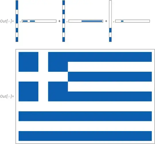
Graphical representation of the solution:
Expand[3 F] /. kp[u__] :> ArrayPlot[KroneckerProduct[u], PlotRangePadding -> None]


ImageData@ColorNegate@Binarize@CountryData["Austria", "Flag"]. – MarcoB Sep 15 '22 at 18:20