Fourier transform of a wave-profile

Question

Hi I tried to do a Fourier transform of a series of points from a plot from ma wave-train profile.

The commands are as such

draupnerpoints= {{-5, 0}, {-4.8, 3}, {-4.5, 1}, {-4.2, 1}, {-4, 3.5}, {-3.8, 
    0}, {-3.5, 6}, {-3.1, 0}, {-3, -5.5}, {-2.8, 0}, {-2.5, 6}, {-2.1,
     0}, {-1.8, -2.5}, {-1.5, 0}, {-1.2, 5}, {-0.8, 
    0}, {-0.5, -8}, {-0.2, 0}, {0, 18}, {1/2, 0}, {2/3, -8}, {1, 
    0}, {4/3, 4}, {3/2, 0}, {1.6, -4}, {2, 3}, {2.5, -3}, {3, 
    3}, {3.2, -2}, {3.5, 2}, {3.8, -4}, {4.2, 0}, {4.5, 
    6}, {4.8, -5}, {5, 0.1}};
ifun = Interpolation[draupnerpoints]
Plot[ifun[[FormalX]], {[FormalX], -5., 5.}, 
 Epilog -> {Red, Point[draupnerpoints]}]

which give

Now, we have the interpolated plot. But since i want to do a Discrete Fourier transform of it, I continue as such:

sr = 3(*sample rate*);
ft = Fourier[draupnerpoints, FourierParameters -> {-1, -1}];
ff = Table[(n - 1) sr/Length@draupnerpoints, {n, 
   Length@draupnerpoints}]

Then I get a series of points, which form a linear function, however this was not as expected. I expected a Fourier-type function which is similar to the plot.

How can I get a Fourier series that represents this plot from the commands issued?

Thanks

ff is a linear sequence,because you constructed it as such. Further, ff is the discrete Fourier transform of a 2D function. Presumably not what you want. Look up the syntax of "Fourier" in the help — Daniel Huber, Nov 23 '22 at 17:49

score 3 · Accepted Answer · answered Nov 23 '22 at 17:35

Here I show how to get a Fourier spectrum from your data. I have put some detailed notes on numerical Fourier transforms here.

First I look at your raw data as follows

    draupnerpoints = {{-5, 0}, {-4.8, 3}, {-4.5, 1}, {-4.2, 1}, {-4, 
    3.5}, {-3.8, 0}, {-3.5, 6}, {-3.1, 0}, {-3, -5.5}, {-2.8, 
    0}, {-2.5, 6}, {-2.1, 0}, {-1.8, -2.5}, {-1.5, 0}, {-1.2, 
    5}, {-0.8, 0}, {-0.5, -8}, {-0.2, 0}, {0, 18}, {1/2, 
    0}, {2/3, -8}, {1, 0}, {4/3, 4}, {3/2, 0}, {1.6, -4}, {2, 
    3}, {2.5, -3}, {3, 3}, {3.2, -2}, {3.5, 2}, {3.8, -4}, {4.2, 
    0}, {4.5, 6}, {4.8, -5}, {5, 0.1}};
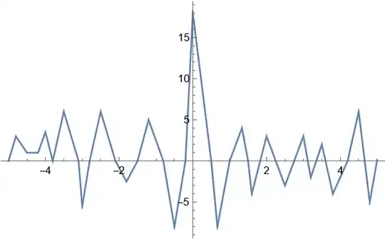
ListLinePlot[draupnerpoints]

This shows that there are about 12 cycles in 10 seconds so a frequency of about 1.2 cycles per second. To re-sample this needs a sample rate of at least about 3 but more would be better. I am going to use 30.

Next I interpolate your data and sample to give me evenly spaced points

sr = 30.; (* Sample rate*)
int = Interpolation[draupnerpoints];
pts = Table[{t, int[t]}, {t, -5, 5, 1/sr}];
Plot[int[t], {t, -5, 5}, Epilog -> {Red, Point[pts]}]

Now we can calculate a spectrum. I first calculate the values of a frequency axis. Then I take the Fourier transform. Finally I calculate the absolute value of the spectral values.

finc = sr/Length[pts]; (* frequency increment *)
ff = Table[f, {f, 0, sr - finc, finc}];
spectrum = 
  Transpose[{ff, 
    Fourier[pts[[All, 2]], FourierParameters -> {-1, -1}]}];
abs = {#[[1]], Abs[#[[2]]]} & /@ spectrum;
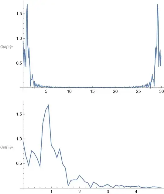
ListLinePlot[abs, PlotRange -> All]
ListLinePlot[abs[[1 ;; 50]], PlotRange -> All]

The first plot shows the whole spectrum. The second the frequency range where your data is located. The frequency peak is actually at about 0.84 Hz so the original estimate of 1.2 Hz was rather high. Note that in the whole spectrum the second half is a mirror image of the first half. These are the negative frequencies. This is because the spectrum is periodic and the tradition is to do the positive frequencies first and the negative second which is fine as the spectrum is periodic.

Hope that helps

Thanks Hugh, this is very interesting answer. Since we are looking at a wavepattern, is your solution decomposing the wavepattern into wave-patterns of other frequencies? — Vangsnes, Nov 23 '22 at 18:02
I was assuming a time history. Is the data a spatial distribution of points? If so the spectrum is in wave numbers not Hz. The decomposition is into sine and cosin waves. — Hugh, Nov 23 '22 at 18:06
Yes, the wave pattern is a timedependent distribution. So your assumption was correct. Is there any way to identify the analytic function of the Fourier transform, as sin and cosine function? — Vangsnes, Nov 23 '22 at 18:20
Yes. The cos terms are given by the real part and the sin terms by the imaginary part. This does not generally get you further since the function is numeric rather than analytic. There is no simple function that would look like your spectrum. If you have some analytic function you believe to model the data you could fit it to the data treating the jagged aspects as noise. — Hugh, Nov 23 '22 at 21:06
Ok, I though that interpolation could have made piecewise function of several analytic approximations along several intervals. — Vangsnes, Nov 24 '22 at 08:50
The interpolation uses cubic spines. There are discontinuities in higher derivatives at each data point that result in branch cuts in the complex plane. See numerical analytic continuattion — Hugh, Nov 24 '22 at 12:06

Fourier transform of a wave-profile

1 Answers1