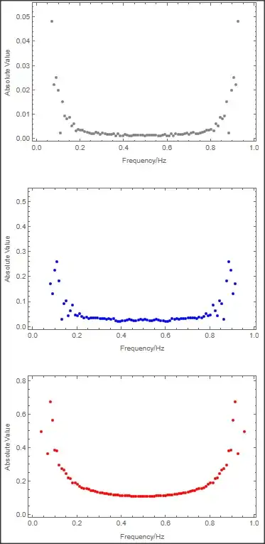
Fourier transform on analogue signal to frequency domain

Question

Hi I have a question regarding the Fourier transform of an analogue signal measured in time domain.

The current 3 data is normalised, and it is expressed in percentage.

I have tried using this line of codes to convert these three analogue signals to the frequency domain. However, it doesn't seem to work. May I ask for some advice on how I can convert these signals to the frequency domain, as I'm the 2nd peak from Data1 could be caused by the signal from Data3, and it would be good to look at the frequency domain. Thanks!

ft = Fourier[Data1, FourierParameters -> {-0, 1}];
sr = 1;
ff = Table[(n - 1) sr/Length[Data1], {n, Length[ft]}] // N;
ListPlot[Transpose[{Data1, Abs[ft]}], PlotRange -> All, 
 Frame -> True, FrameLabel -> {"Frequency/Hz", "Absolute Value"}, 
 PlotStyle -> Gray]
ft = Fourier[Data2, FourierParameters -> {-0, 1}];
sr = 1;
ff = Table[(n - 1) sr/Length[Data2], {n, Length[ft]}] // N;
ListPlot[Transpose[{Data2, Abs[ft]}], PlotRange -> All, 
 Frame -> True, FrameLabel -> {"Frequency/Hz", "Absolute Value"}, 
 PlotStyle -> Blue]
ft = Fourier[Data3, FourierParameters -> {0, 1}];
sr = 1;
ff = Table[(n - 1) sr/Length[Data3], {n, Length[ft]}] // N;
ListPlot[Transpose[{Data3, Abs[ft]}], PlotRange -> All, 
 Frame -> True, FrameLabel -> {"Frequency/Hz", "Absolute Value"}, 
 PlotStyle -> Red]

Data1={{50/49, 0.709518}, {100/49, 0.719227}, {150/49, 0.726746}, {200/49, 0.725896}, {250/49, 0.715706}, {300/49, 0.701223}, {50/7, 0.685712}, {400/49, 0.676085}, {450/49, 0.674719}, {500/49,0.679336}, {550/49, 0.686554}, {600/49, 0.692027}, {650/49, 0.692589}, {100/7, 0.686457}, {750/49, 0.677379}, {800/49, 0.66802}, {850/49, 0.658175}, {900/49, 0.64764}, {950/49, 0.636723}, {1000/49, 0.622386}, {150/7, 0.608827}, {1100/49, 0.594966}, {1150/49, 0.581673}, {1200/49, 0.572631}, {1250/49, 0.567133}, {1300/49, 0.5649}, {1350/49, 0.566716}, {200/7, 0.567491}, {1450/49, 0.56886}, {1500/49, 0.569235}, {1550/49, 0.567608}, {1600/49, 0.564991}, {1650/49, 0.561072}, {1700/49, 0.557299}, {250/7, 0.555122}, {1800/49, 0.555683}, {1850/49, 0.558299}, {1900/49, 0.562949}, {1950/49, 0.568865}, {2000/49, 0.57652}, {2050/49, 0.58673}, {300/7, 0.601072}, {2150/49, 0.620133}, {2200/49, 0.642991}, {2250/49, 0.669782}, {2300/49, 0.698904}, {2350/49, 0.731528}, {2400/49, 0.768227}, {50, 0.810462}, {2500/49, 0.857938}, {2550/49, 0.91105}, {2600/49, 0.97133}, {2650/49, 1.03985}, {2700/49, 1.11519}, {2750/49, 1.19911}, {400/7, 1.28624}, {2850/49, 1.37416}, {2900/49, 1.4627}, {2950/49, 1.54656}, {3000/49, 1.62408}, {3050/49, 1.69271}, {3100/49, 1.74688}, {450/7, 1.78762}, {3200/49, 1.81292}, {3250/49, 1.8254}, {3300/49, 1.82721}, {3350/49, 1.81656}, {3400/49, 1.79814}, {3450/49, 1.77086}, {500/7, 1.73145}, {3550/49, 1.68872}, {3600/49, 1.64251}, {3650/49, 1.5951}, {3700/49, 1.55741}, {3750/49, 1.52962}, {3800/49, 1.51497}, {550/7, 1.50966}, {3900/49, 1.50824}, {3950/49, 1.50322}, {4000/49, 1.48808}, {4050/49, 1.45785}, {4100/49, 1.41212}, {4150/49, 1.35233}, {600/7, 1.27981}, {4250/49, 1.19999}, {4300/49, 1.11879}, {4350/49, 1.03842}, {4400/49, 0.963963}, {4450/49, 0.897695}, {4500/49, 0.840438}, {650/7,0.793229}, {4600/49, 0.757297}, {4650/49, 0.73282}, {4700/49, 0.720508}, {4750/49, 0.718504}, {4800/49, 0.72323}, {4850/49, 0.729212}, {100, 0.729535}};

Data2={{50/49, 1.8203}, {100/49, 2.05732}, {150/49, 2.29564}, {200/49, 2.48521}, {250/49, 2.612}, {300/49, 2.71799}, {50/7, 2.79892}, {400/49, 2.84231}, {450/49, 2.85008}, {500/49, 2.85519}, {550/49, 2.85635}, {600/49, 2.8809}, {650/49, 2.8877}, {100/7, 2.87008}, {750/49, 2.85947}, {800/49, 2.81734}, {850/49, 2.76421}, {900/49, 2.69368}, {950/49, 2.60323}, {1000/49, 2.50318}, {150/7, 2.39164}, {1100/49, 2.28347}, {1150/49, 2.20035}, {1200/49, 2.11981}, {1250/49, 2.04034}, {1300/49, 1.96782}, {1350/49, 1.88855}, {200/7, 1.82167}, {1450/49, 1.75124}, {1500/49, 1.68388}, {1550/49, 1.62663}, {1600/49, 1.57906}, {1650/49, 1.54306}, {1700/49, 1.53892}, {250/7, 1.54906}, {1800/49, 1.59038}, {1850/49, 1.66962}, {1900/49, 1.78076}, {1950/49, 1.9356}, {2000/49, 2.12964}, {2050/49, 2.36343}, {300/7, 2.64274}, {2150/49, 2.94583}, {2200/49, 3.28908}, {2250/49, 3.66972}, {2300/49, 4.1053}, {2350/49, 4.60978}, {2400/49, 5.19387}, {50, 5.8709}, {2500/49, 6.66846}, {2550/49, 7.58843}, {2600/49, 8.63363}, {2650/49, 9.82267}, {2700/49, 11.1445}, {2750/49, 12.5993}, {400/7, 14.1672}, {2850/49, 15.8302}, {2900/49, 17.5577}, {2950/49, 19.3084}, {3000/49, 21.0391}, {3050/49, 22.7226}, {3100/49, 24.3202}, {450/7, 25.7954}, {3200/49, 27.1832}, {3250/49, 28.4791}, {3300/49, 29.6025}, {3350/49, 30.441}, {3400/49, 30.8624}, {3450/49, 30.8442}, {500/7, 30.4553}, {3550/49, 29.7744}, {3600/49, 28.8903}, {3650/49, 27.827}, {3700/49, 26.6272}, {3750/49, 25.2827}, {3800/49, 23.8154}, {550/7, 22.2279}, {3900/49, 20.5494}, {3950/49, 18.7886}, {4000/49, 16.9938}, {4050/49, 15.2019}, {4100/49, 13.4352}, {4150/49, 11.7194}, {600/7, 10.0284}, {4250/49, 8.40037}, {4300/49, 6.82511}, {4350/49, 5.33063}, {4400/49, 3.95389}, {4450/49, 2.75903},{4500/49, 1.78265}, {650/7, 1.06054}, {4600/49, 0.620857}, {4650/49, 0.47017}, {4700/49, 0.505546}, {4750/49, 0.695713}, {4800/49, 0.874938}, {4850/49, 1.0074}, {100, 1.16654}};

Data3={{50/49, 0.0581721}, {100/49, 0.416446}, {150/49, 0.725649}, {200/49, 0.983077}, {250/49, 1.19155}, {300/49, 1.3719}, {50/7, 1.53917}, {400/49, 1.70562}, {450/49, 1.88342}, {500/49, 2.07945}, {550/49, 2.29185}, {600/49, 2.51525}, {650/49, 2.73457}, {100/7, 2.93913}, {750/49, 3.12689}, {800/49, 3.29443}, {850/49, 3.44589}, {900/49, 3.58164}, {950/49, 3.71092}, {1000/49, 3.8268}, {150/7, 3.92081}, {1100/49, 3.98627}, {1150/49, 4.01713}, {1200/49, 4.02147}, {1250/49, 4.00736}, {1300/49, 3.98636}, {1350/49, 3.96508}, {200/7, 3.95175}, {1450/49, 3.95412}, {1500/49, 3.97308}, {1550/49, 4.00978}, {1600/49, 4.05879}, {1650/49, 4.1227}, {1700/49, 4.19884}, {250/7, 4.28635}, {1800/49, 4.37801}, {1850/49, 4.46369}, {1900/49, 4.53319}, {1950/49, 4.58796}, {2000/49, 4.6351}, {2050/49, 4.66959}, {300/7, 4.67729}, {2150/49, 4.65765}, {2200/49, 4.61185}, {2250/49, 4.5271}, {2300/49, 4.39923}, {2350/49, 4.23296}, {2400/49, 4.03914}, {50, 3.81889}, {2500/49, 3.56881}, {2550/49, 3.29911}, {2600/49, 3.00481}, {2650/49, 2.66873}, {2700/49, 2.27429}, {2750/49, 1.81681}, {400/7, 1.3059}, {2850/49, 0.762932}, {2900/49, 0.210746}, {2950/49, -0.324365}, {3000/49, -0.823801}, {3050/49, -1.26847}, {3100/49, -1.65267}, {450/7, -1.98326}, {3200/49, -2.28159}, {3250/49, -2.56956}, {3300/49, -2.87368}, {3350/49, -3.20578}, {3400/49, -3.56684}, {3450/49, -3.95302}, {500/7, -4.33628}, {3550/49, -4.70217}, {3600/49, -5.04992}, {3650/49, -5.35797}, {3700/49, -5.6026}, {3750/49, -5.79287}, {3800/49, -5.94693}, {550/7, -6.05814}, {3900/49, -6.11988}, {3950/49, -6.14301}, {4000/49, -6.14404}, {4050/49, -6.11633}, {4100/49, -6.05179}, {4150/49, -5.94962}, {600/7, -5.80898}, {4250/49, -5.63541}, {4300/49, -5.43704}, {4350/49, -5.21484}, {4400/49, -4.97545}, {4450/49, -4.7302}, {4500/49, -4.48732}, {650/7, -4.24384}, {4600/49, -4.00672}, {4650/49, -3.78217}, {4700/49, -3.56916}, {4750/49, -3.34286}, {4800/49, -3.06888}, {4850/49, -2.74621}, {100, -2.38982}};

I have put some notes on using Fourier here hope they help. – Hugh Dec 06 '22 at 09:06 — Hugh, Dec 06 '22 at 09:06

Daniel Huber · Answer 1 · 2022-12-08T15:35:35.397

For "Fourier", you only need the vector of measured data, not the time. The vector of frequencies corresponds to normalized frequencies: 0...0.5...0. The first half corresponds to negative frequencies: Exp[-I f t], the second half to positiveones: Exp[+I f t]. "0.5" corresponds to the highest frequency that you can sample, namely 2 measured points in a period. Higher frequencies can not be distinguished from lower ones (see Nyquist theorem).

With this:

ft = Fourier[Data1[[All, 2]], FourierParameters -> {-0, 1}];
sr = 1;
ff = Table[(n - 1) sr/Length[Data1], {n, Length[ft]}] // N;
ListPlot[Transpose[{ff, Abs[ft]}], PlotRange -> All, Frame -> True, 
 FrameLabel -> {"Frequency/Hz", "Absolute Value"}, PlotStyle -> Gray]
ft = Fourier[Data2[[All, 2]], FourierParameters -> {-0, 1}];
sr = 1;
ff = Table[(n - 1) sr/Length[Data2], {n, Length[ft]}] // N;
ListPlot[Transpose[{ff, Abs[ft]}], PlotRange -> All, Frame -> True, 
 FrameLabel -> {"Frequency/Hz", "Absolute Value"}, PlotStyle -> Blue]
ft = Fourier[Data3[[All, 2]], FourierParameters -> {0, 1}];
sr = 1;
ff = Table[(n - 1) sr/Length[Data3], {n, Length[ft]}] // N;
ListPlot[Transpose[{ff, Abs[ft]}], PlotRange -> All, Frame -> True, 
 FrameLabel -> {"Frequency/Hz", "Absolute Value"}, PlotStyle -> Red]

As you see, the plot is dominated by the 0 frequency. Therefore, it make sense, to delete "PlotRange->All":

Fourier transform on analogue signal to frequency domain

1 Answers1